Nested Forecasting Approach and modeltime Methods

class: center, middle, inverse, title-slide

.title[
# Nested Forecasting Approach and modeltime Methods
]
.author[
### Dr. Kam Tin Seong Assoc. Professor of Information Systems
]
.institute[
### School of Computing and Information Systems, Singapore Management University
]
.date[
### 2022-7-16 (updated: 2022-07-30)
]

---

# Content

.vlarge[
+ The motivation 
+ Principles of nested forecasting approach
+ Nested forecasting processes
+ Nested forecasting with modeltime
]

---
## Motivation of Nested Forecasting Approach

.large[
In real world practice, it is very common a forecaster is required to forecast multiple time series by fitting multiple models.
]

.center[
![:scale 65%](img/image21.png)]

---
class: center, middle

# Nested Forecasting

![:scale 40%](img/image18.jpg)

.small[
Source: [Getting Started with Modeltime](https://business-science.github.io/modeltime/articles/nested-forecasting.html)
]

---
## Setting Up R Environment

.pull-left[
For the purpose of this hands-on exercise, the following R packages will be used.

```r
pacman::p_load(tidyverse, tidymodels, 
               timetk, modeltime)
```

+ [**tidyverse**](https://lubridate.tidyverse.org/) provides a collection of commonly used functions for importing, wrangling and visualising data.  In this hands-on exercise the main packages used are readr, dplyr, tidyr and ggplot2.  
]

.pull-right[
+ [**modeltime**](https://business-science.github.io/modeltime/index.html) a new time series forecasting package designed to speed up model evaluation, selection, and forecasting. modeltime does this by integrating the [**tidymodels**](https://www.tidymodels.org/) machine learning ecosystem of packages into a streamlined workflow for tidyverse
forecasting. 
]

---
## The data

.pull-left[
In this sharing, [**Store Sales - Time Series Forecasting: Use machine learning to predict grocery sales**](https://www.kaggle.com/competitions/store-sales-time-series-forecasting/overview) from Kaggle competition will be used.  For the purpose of this sharing, the main data set used is *train.csv*.  It consists of six columns.  They are:

+ *id* contains unique id for each records.
+ *date* gives the sales dates.
+ *store_nbr* identifies the store at which the products are sold.
+ *family* identifies the type of product sold.
+ *sales* gives the total sales for a product family at a particular store at a given date. Fractional values are possible since products can be sold in fractional units (1.5 kg of cheese, for instance, as opposed to 1 bag of chips).
+ *onpromotion* gives the total number of items in a product family that were being promoted at a store at a given date.
]

--
.pull-right[
For the purpose of this sharing, I will focus of grocery sales instead of all products.  Code chunk below is used to extract grocery sales from *train.csv* and saved the output into an rds file format for subsequent used.

```r
grocery <- read_csv(
 "data/store_sales/train.csv") %>%
 filter(family == "GROCERY") %>%
 write_rds(
 "data/store_sales/grocery.rds")
```
]

---
### Step 1: Data Import and Wrangling

.pull-left[
In the code chunk below, `read_rds()` of **readr** package is used to import grocery.rds data into R environment. Then, `mutate()`, `across()` and `as.factor()` are used to convert all values in columns 1,3 and 4 into factor data type.

```r
grocery <- read_rds(
 "data/store_sales/grocery.rds") %>%
 mutate(across(c(1, 3, 4), 
 as.factor)) %>%
 filter(date >= "2015-01-01")
```
]

--
.pull-right[
In the code chunk below, `read_csv()` is used to import *stores.csv* file into R environment.  TThen, `mutate()`, `across()` and `as.factor()` are used to convert values in columns 1to 5 into factor data type.

```r
stores <- read_csv(
 "data/store_sales/stores.csv") %>%
 mutate(across(c(1:5), 
 as.factor)) %>%
 select(store_nbr, cluster)
```
]

---
### Data integration and wrangling

.pull-left[
In the code chunk below, `left_join()` of **dplyr** package is used to join *grocery* and *stores* tibble data frames by using *store_nb*r as unique field.

```r
grocery_stores <- left_join(
 x = grocery,
 y = stores,
 by = "store_nbr")
```
]

--
.pull-right[
In the code chunk below, a new tibble data frame called *grocery_cluster* is derived by summing sales values by values in cluster and date fields.

```r
grocery_cluster <- grocery_stores %>%
 group_by(cluster, date) %>%
 summarise(value = sum(sales)) %>%
 select(cluster, date, value) %>%
 set_names(c("id", "date", "value")) %>%
 ungroup()
```
]

---
### Visualising the time series data: The code chunk

.pull-left[
It is always a good practice to visualise the time series graphically.

```r
grocery_cluster %>%
  group_by(id) %>%
  plot_time_series(
    date, value,
    .line_size = 0.4,
    .facet_ncol = 5, 
    .facet_scales = "free_y",
    .interactive = FALSE,
    .smooth_size = 0.4)
```
]

---
### Visualising the time series data: The plot

![:scale 70%](img/image21.png)

---
## Preparation for Nested Forecasting

.pull-left[
Before fitting the nested forecasting models, there are two key components that we need to prepare for:

+ **Nested Data Structure:** Most critical to ensure your data is prepared (covered next).
+ **Nested Modeltime Workflow:** This stage is where we create many models, fit the models to the data, and generate forecasts at scale.
]

.pull-right[
![](img/image19.jpg)
]

---
### Step 2: Preparing Nested Time Series Data Frame

.pull-left[
.large[
There are three major steps in reparing the nested time series data frame.  They are:

+ Creating an initial data frame and extending to the future,

+ Transforming the tibble data frame into nested modeltime data frame, and

+ Splitting the nested data frame into training and test (hold-out) data sets.
]]

---
### **Creating initial data frame and extending to the future**

.pull-left[
Firstly, we will create a new data table and extend the time frame 60 days into the future by using [`extend_timeseries()`](https://business-science.github.io/modeltime/reference/prep_nested.html) of modeltime.

```r
nested_tbl <- grocery_cluster %>%
 extend_timeseries(
 .id_var = id,
 .date_var = date,
 .length_future = "60 days") 
```
]

.pull-right[
![:scale 40%](img/image22.jpg)
]

---
### Nesting the tibble data frame
 
.pull-left[
Next, [`nest_timeseries()`](https://business-science.github.io/modeltime/reference/prep_nested.html) is used to transform the newly created data frame in previous slide into a  nested data frame by grouping the values in the *id* field.

```r
nested_tbl <- nested_tbl %>%
 nest_timeseries(
 .id_var = id,
 .length_future = 60,
 .length_actual = 17272) 
```

Notice that the nested data frame consists of three fields namely *id*, *.actual_data* and *.future_data*.]

.pull-right[
![:scale 55%](img/image23.jpg)
]

---
### Data sampling

.pull-left[
Lastly, `split_nested_timeseries()` is used to split the original data into training and testing (or hold-out) data sets.

```r
nested_tbl <- nested_tbl %>%
 split_nested_timeseries(
 .length_test = 60)
```
]

.pull-right[
![](img/image24.jpg)
]

---
### Step 3: Creating Tidymodels Workflows

In this step, we will first applying tidymodels approach to create four forecasting models by using [`recipe()`](https://recipes.tidymodels.org/reference/recipe.html) of [**recipe**](https://recipes.tidymodels.org/) package and [`workflow()`](https://workflows.tidymodels.org/reference/workflow.html) of [**workflow**](https://workflows.tidymodels.org/) package. Both packages are member of [**tidymodels**](https://www.tidymodels.org/), a family of R packages specially designed for  modeling and machine learning using [**tidyverse**](https://www.tidyverse.org/) principles.

.pull-left[
**Model 1: Exponential Smoothing (Modeltime)**

An Error-Trend-Season (ETS) model by using [`exp_smoothing()`](https://business-science.github.io/modeltime/reference/exp_smoothing.html).

```r
rec_autoETS <- recipe(
 value ~ date, 
 extract_nested_train_split(
 nested_tbl))

wflw_autoETS <- workflow() %>%
 add_model(
 exp_smoothing() %>% 
 set_engine("ets")) %>%
 add_recipe(rec_autoETS)
```
]

--
.pull-right[
**Model 2: Auto ARIMA (Modeltime)**

An auto ARIMA model by using [`arima_reg()`](https://business-science.github.io/modeltime/reference/arima_reg.html).

```r
rec_autoARIMA <- recipe(
 value ~ date, 
 extract_nested_train_split(
 nested_tbl))

wflw_autoARIMA <- workflow() %>%
 add_model(
 arima_reg() %>% 
 set_engine("auto_arima")) %>%
 add_recipe(rec_autoARIMA)
```
]

---
### Step 3: Creating Tidymodels Workflows (cont')
.pull-left[

**Model 3: Boosted Auto ARIMA (Modeltime)**

An Boosted auto ARIMA model by using [`arima_boost()`](https://business-science.github.io/modeltime/reference/arima_boost.html).

```r
rec_xgb <- recipe(
 value ~ .,
 extract_nested_train_split(
 nested_tbl)) %>%
 step_timeseries_signature(date) %>%
 step_rm(date) %>%
 step_zv(all_predictors()) %>%
 step_dummy(all_nominal_predictors(), 
 one_hot = TRUE)

wflw_xgb <- workflow() %>%
 add_model(
 boost_tree(
 "regression") %>% 
 set_engine("xgboost")) %>%
 add_recipe(rec_xgb)
```
]

--
.pull-right[
**Model 4: prophet (Modeltime)**

A prophet model using [`prophet_reg()`](https://business-science.github.io/modeltime/reference/prophet_reg.html).

```r
rec_prophet <- recipe(
 value ~ date, 
 extract_nested_train_split(
 nested_tbl))

wflw_prophet <- workflow() %>%
 add_model(
 prophet_reg(
 "regression", 
 seasonality_yearly = TRUE) %>%
 set_engine("prophet")
 ) %>%
 add_recipe(rec_prophet)
```
]

---
### Prophet

[**Prophet**](https://facebook.github.io/prophet/) is a procedure for forecasting time series data based on an additive model where non-linear trends are fit with yearly, weekly, and daily seasonality, plus holiday effects. The general formula is defined as follow:

![](img/image29.png)

It works best with time series that have strong seasonal effects and several seasons of historical data. Prophet is robust to missing data and shifts in the trend, and typically handles outliers well.

.small[
Source: [Forecasting at Scale](https://peerj.com/preprints/3190/)
]

---
### XGBoost forecasting algorithm

**XGBoost(Extreme Gradient Boosting)** is an implementation of the gradient boosting ensemble algorithm for classification and regression. Time series datasets can be transformed into supervised learning using a sliding-window representation.

![:scale 70%](img/image30.png)

.small[
Reference: [XGBOOST AS A TIME-SERIES
FORECASTING TOOL](https://filip-wojcik.com/talks/xgboost_forecasting_eng.pdf)
]

---
### What is so special of XGBoost?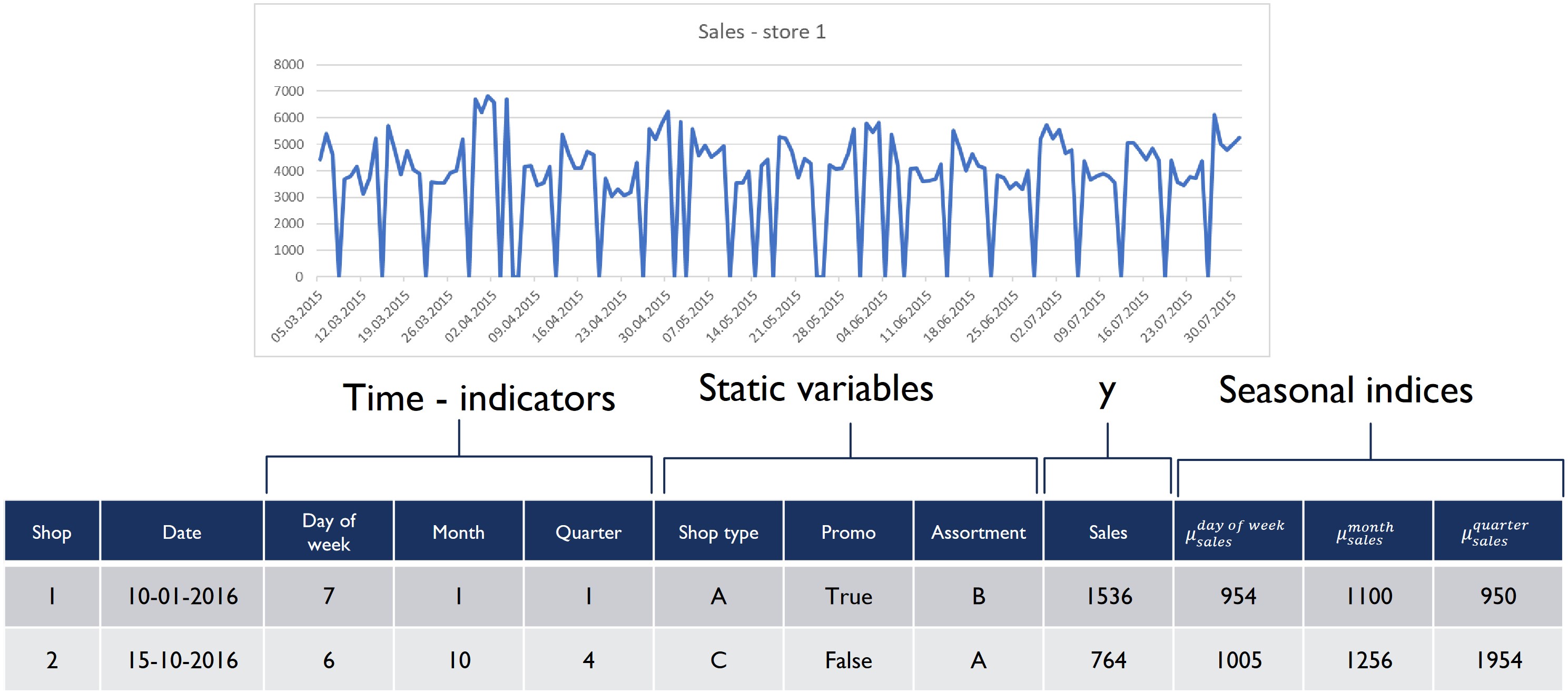

![](img/image31.jpg)

---
## Nested Forecasting with modeltime

.center[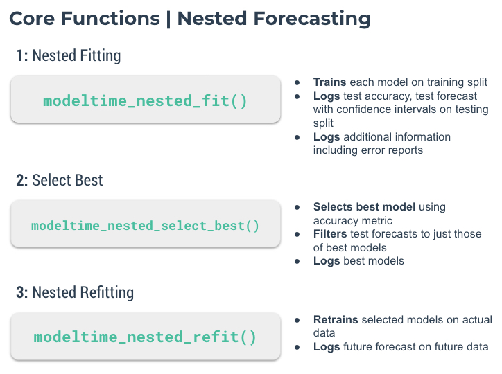
![:scale 50%](img/image20.jpg)]

---
### Step 4: Fitting Nested Forecasting Models

.pull-left[
In this step, [`modeltime_nested_fit()`](https://business-science.github.io/modeltime/reference/modeltime_nested_fit.html) is used to fit the four models we created in Step 3.  Note that the input must be in the form of nested modeltime table (i.e. *nested_tbl*)

```r
nested_tbl <- modeltime_nested_fit(
 nested_data = nested_tbl,
 wflw_autoETS,
 wflw_autoARIMA,
 wflw_prophet,
 wflw_xgb)
```
]

---
### The nested modeltime data frame

The output object *nested_tbl* is a nested modetime data frame.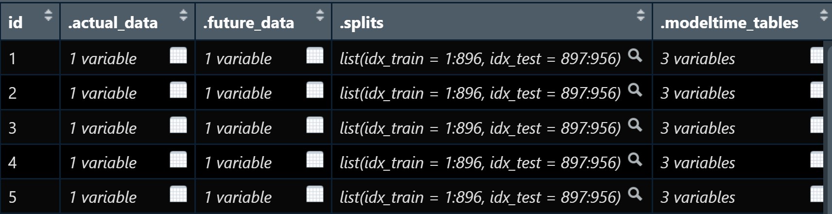

![:scale 65%](img/image25a.jpg)

Click on the table icon of the first row under *.modeltime_tables* field, its corresponding modelling data frame appears.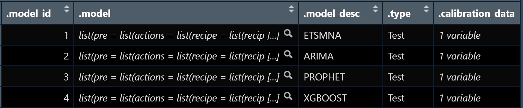

![:scale 70%](img/image25b.jpg)

Notice that the four models were fitted by using the test data set.

---
### Step 5: Model Accuracy Assessment with Test Logged Attributes

.pull-left[
Before we go ahead to select the best model, it is a good practice to compare the performance of the models by using accuracy matrices.

```r
nested_tbl %>%
  extract_nested_test_accuracy() %>%
  table_modeltime_accuracy(
    .interactive = FALSE)
```

What can we learn fro mthe code chunk above?

+ [`extract_nested_test_accuracy()`](https://business-science.github.io/modeltime/reference/log_extractors.html) is used to extract the accuracy matrices by using the test data set.

+ [`table_modeltime_accuracy()`](https://business-science.github.io/modeltime/reference/table_modeltime_accuracy.html) is used to display the accuracy report in tabular form.
]

.pull-right[
Note that `.interactive` argument returns interactive or static tables. If TRUE, returns `reactable` table. If FALSE, returns static `gt` table.
]

---
### Step 5: Model Accuracy Assessment with Test Logged Attributes

<div id="mehsihgtqz" style="overflow-x:auto;overflow-y:auto;width:auto;height:auto;">
<style>html {
 font-family: -apple-system, BlinkMacSystemFont, 'Segoe UI', Roboto, Oxygen, Ubuntu, Cantarell, 'Helvetica Neue', 'Fira Sans', 'Droid Sans', Arial, sans-serif;
}

#mehsihgtqz .gt_table {
  display: table;
  border-collapse: collapse;
  margin-left: auto;
  margin-right: auto;
  color: #333333;
  font-size: 16px;
  font-weight: normal;
  font-style: normal;
  background-color: #FFFFFF;
  width: auto;
  border-top-style: solid;
  border-top-width: 2px;
  border-top-color: #A8A8A8;
  border-right-style: none;
  border-right-width: 2px;
  border-right-color: #D3D3D3;
  border-bottom-style: solid;
  border-bottom-width: 2px;
  border-bottom-color: #A8A8A8;
  border-left-style: none;
  border-left-width: 2px;
  border-left-color: #D3D3D3;
}

#mehsihgtqz .gt_heading {
  background-color: #FFFFFF;
  text-align: center;
  border-bottom-color: #FFFFFF;
  border-left-style: none;
  border-left-width: 1px;
  border-left-color: #D3D3D3;
  border-right-style: none;
  border-right-width: 1px;
  border-right-color: #D3D3D3;
}

#mehsihgtqz .gt_title {
  color: #333333;
  font-size: 125%;
  font-weight: initial;
  padding-top: 4px;
  padding-bottom: 4px;
  padding-left: 5px;
  padding-right: 5px;
  border-bottom-color: #FFFFFF;
  border-bottom-width: 0;
}

#mehsihgtqz .gt_subtitle {
  color: #333333;
  font-size: 85%;
  font-weight: initial;
  padding-top: 0;
  padding-bottom: 6px;
  padding-left: 5px;
  padding-right: 5px;
  border-top-color: #FFFFFF;
  border-top-width: 0;
}

#mehsihgtqz .gt_bottom_border {
  border-bottom-style: solid;
  border-bottom-width: 2px;
  border-bottom-color: #D3D3D3;
}

#mehsihgtqz .gt_col_headings {
  border-top-style: solid;
  border-top-width: 2px;
  border-top-color: #D3D3D3;
  border-bottom-style: solid;
  border-bottom-width: 2px;
  border-bottom-color: #D3D3D3;
  border-left-style: none;
  border-left-width: 1px;
  border-left-color: #D3D3D3;
  border-right-style: none;
  border-right-width: 1px;
  border-right-color: #D3D3D3;
}

#mehsihgtqz .gt_col_heading {
  color: #333333;
  background-color: #FFFFFF;
  font-size: 100%;
  font-weight: normal;
  text-transform: inherit;
  border-left-style: none;
  border-left-width: 1px;
  border-left-color: #D3D3D3;
  border-right-style: none;
  border-right-width: 1px;
  border-right-color: #D3D3D3;
  vertical-align: bottom;
  padding-top: 5px;
  padding-bottom: 6px;
  padding-left: 5px;
  padding-right: 5px;
  overflow-x: hidden;
}

#mehsihgtqz .gt_column_spanner_outer {
  color: #333333;
  background-color: #FFFFFF;
  font-size: 100%;
  font-weight: normal;
  text-transform: inherit;
  padding-top: 0;
  padding-bottom: 0;
  padding-left: 4px;
  padding-right: 4px;
}

#mehsihgtqz .gt_column_spanner_outer:first-child {
  padding-left: 0;
}

#mehsihgtqz .gt_column_spanner_outer:last-child {
  padding-right: 0;
}

#mehsihgtqz .gt_column_spanner {
  border-bottom-style: solid;
  border-bottom-width: 2px;
  border-bottom-color: #D3D3D3;
  vertical-align: bottom;
  padding-top: 5px;
  padding-bottom: 5px;
  overflow-x: hidden;
  display: inline-block;
  width: 100%;
}

#mehsihgtqz .gt_group_heading {
  padding-top: 8px;
  padding-bottom: 8px;
  padding-left: 5px;
  padding-right: 5px;
  color: #333333;
  background-color: #FFFFFF;
  font-size: 100%;
  font-weight: initial;
  text-transform: inherit;
  border-top-style: solid;
  border-top-width: 2px;
  border-top-color: #D3D3D3;
  border-bottom-style: solid;
  border-bottom-width: 2px;
  border-bottom-color: #D3D3D3;
  border-left-style: none;
  border-left-width: 1px;
  border-left-color: #D3D3D3;
  border-right-style: none;
  border-right-width: 1px;
  border-right-color: #D3D3D3;
  vertical-align: middle;
}

#mehsihgtqz .gt_empty_group_heading {
  padding: 0.5px;
  color: #333333;
  background-color: #FFFFFF;
  font-size: 100%;
  font-weight: initial;
  border-top-style: solid;
  border-top-width: 2px;
  border-top-color: #D3D3D3;
  border-bottom-style: solid;
  border-bottom-width: 2px;
  border-bottom-color: #D3D3D3;
  vertical-align: middle;
}

#mehsihgtqz .gt_from_md > :first-child {
  margin-top: 0;
}

#mehsihgtqz .gt_from_md > :last-child {
  margin-bottom: 0;
}

#mehsihgtqz .gt_row {
  padding-top: 8px;
  padding-bottom: 8px;
  padding-left: 5px;
  padding-right: 5px;
  margin: 10px;
  border-top-style: solid;
  border-top-width: 1px;
  border-top-color: #D3D3D3;
  border-left-style: none;
  border-left-width: 1px;
  border-left-color: #D3D3D3;
  border-right-style: none;
  border-right-width: 1px;
  border-right-color: #D3D3D3;
  vertical-align: middle;
  overflow-x: hidden;
}

#mehsihgtqz .gt_stub {
  color: #333333;
  background-color: #FFFFFF;
  font-size: 100%;
  font-weight: initial;
  text-transform: inherit;
  border-right-style: solid;
  border-right-width: 2px;
  border-right-color: #D3D3D3;
  padding-left: 5px;
  padding-right: 5px;
}

#mehsihgtqz .gt_stub_row_group {
  color: #333333;
  background-color: #FFFFFF;
  font-size: 100%;
  font-weight: initial;
  text-transform: inherit;
  border-right-style: solid;
  border-right-width: 2px;
  border-right-color: #D3D3D3;
  padding-left: 5px;
  padding-right: 5px;
  vertical-align: top;
}

#mehsihgtqz .gt_row_group_first td {
  border-top-width: 2px;
}

#mehsihgtqz .gt_summary_row {
  color: #333333;
  background-color: #FFFFFF;
  text-transform: inherit;
  padding-top: 8px;
  padding-bottom: 8px;
  padding-left: 5px;
  padding-right: 5px;
}

#mehsihgtqz .gt_first_summary_row {
  border-top-style: solid;
  border-top-color: #D3D3D3;
}

#mehsihgtqz .gt_first_summary_row.thick {
  border-top-width: 2px;
}

#mehsihgtqz .gt_last_summary_row {
  padding-top: 8px;
  padding-bottom: 8px;
  padding-left: 5px;
  padding-right: 5px;
  border-bottom-style: solid;
  border-bottom-width: 2px;
  border-bottom-color: #D3D3D3;
}

#mehsihgtqz .gt_grand_summary_row {
  color: #333333;
  background-color: #FFFFFF;
  text-transform: inherit;
  padding-top: 8px;
  padding-bottom: 8px;
  padding-left: 5px;
  padding-right: 5px;
}

#mehsihgtqz .gt_first_grand_summary_row {
  padding-top: 8px;
  padding-bottom: 8px;
  padding-left: 5px;
  padding-right: 5px;
  border-top-style: double;
  border-top-width: 6px;
  border-top-color: #D3D3D3;
}

#mehsihgtqz .gt_striped {
  background-color: rgba(128, 128, 128, 0.05);
}

#mehsihgtqz .gt_table_body {
  border-top-style: solid;
  border-top-width: 2px;
  border-top-color: #D3D3D3;
  border-bottom-style: solid;
  border-bottom-width: 2px;
  border-bottom-color: #D3D3D3;
}

#mehsihgtqz .gt_footnotes {
  color: #333333;
  background-color: #FFFFFF;
  border-bottom-style: none;
  border-bottom-width: 2px;
  border-bottom-color: #D3D3D3;
  border-left-style: none;
  border-left-width: 2px;
  border-left-color: #D3D3D3;
  border-right-style: none;
  border-right-width: 2px;
  border-right-color: #D3D3D3;
}

#mehsihgtqz .gt_footnote {
  margin: 0px;
  font-size: 90%;
  padding-left: 4px;
  padding-right: 4px;
  padding-left: 5px;
  padding-right: 5px;
}

#mehsihgtqz .gt_sourcenotes {
  color: #333333;
  background-color: #FFFFFF;
  border-bottom-style: none;
  border-bottom-width: 2px;
  border-bottom-color: #D3D3D3;
  border-left-style: none;
  border-left-width: 2px;
  border-left-color: #D3D3D3;
  border-right-style: none;
  border-right-width: 2px;
  border-right-color: #D3D3D3;
}

#mehsihgtqz .gt_sourcenote {
  font-size: 90%;
  padding-top: 4px;
  padding-bottom: 4px;
  padding-left: 5px;
  padding-right: 5px;
}

#mehsihgtqz .gt_left {
  text-align: left;
}

#mehsihgtqz .gt_center {
  text-align: center;
}

#mehsihgtqz .gt_right {
  text-align: right;
  font-variant-numeric: tabular-nums;
}

#mehsihgtqz .gt_font_normal {
  font-weight: normal;
}

#mehsihgtqz .gt_font_bold {
  font-weight: bold;
}

#mehsihgtqz .gt_font_italic {
  font-style: italic;
}

#mehsihgtqz .gt_super {
  font-size: 65%;
}

#mehsihgtqz .gt_two_val_uncert {
  display: inline-block;
  line-height: 1em;
  text-align: right;
  font-size: 60%;
  vertical-align: -0.25em;
  margin-left: 0.1em;
}

#mehsihgtqz .gt_footnote_marks {
  font-style: italic;
  font-weight: normal;
  font-size: 75%;
  vertical-align: 0.4em;
}

#mehsihgtqz .gt_asterisk {
  font-size: 100%;
  vertical-align: 0;
}

#mehsihgtqz .gt_slash_mark {
  font-size: 0.7em;
  line-height: 0.7em;
  vertical-align: 0.15em;
}

#mehsihgtqz .gt_fraction_numerator {
  font-size: 0.6em;
  line-height: 0.6em;
  vertical-align: 0.45em;
}

#mehsihgtqz .gt_fraction_denominator {
 font-size: 0.6em;
 line-height: 0.6em;
 vertical-align: -0.05em;
}
</style>
<table class="gt_table">
 <thead class="gt_header">
 <tr>
 <th colspan="10" class="gt_heading gt_title gt_font_normal gt_bottom_border" style>Accuracy Table</th>
 </tr>
 
 </thead>
 <thead class="gt_col_headings">
 <tr>
 <th class="gt_col_heading gt_columns_bottom_border gt_center" rowspan="1" colspan="1">id</th>
 <th class="gt_col_heading gt_columns_bottom_border gt_right" rowspan="1" colspan="1">.model_id</th>
 <th class="gt_col_heading gt_columns_bottom_border gt_left" rowspan="1" colspan="1">.model_desc</th>
 <th class="gt_col_heading gt_columns_bottom_border gt_left" rowspan="1" colspan="1">.type</th>
 <th class="gt_col_heading gt_columns_bottom_border gt_right" rowspan="1" colspan="1">mae</th>
 <th class="gt_col_heading gt_columns_bottom_border gt_right" rowspan="1" colspan="1">mape</th>
 <th class="gt_col_heading gt_columns_bottom_border gt_right" rowspan="1" colspan="1">mase</th>
 <th class="gt_col_heading gt_columns_bottom_border gt_right" rowspan="1" colspan="1">smape</th>
 <th class="gt_col_heading gt_columns_bottom_border gt_right" rowspan="1" colspan="1">rmse</th>
 <th class="gt_col_heading gt_columns_bottom_border gt_right" rowspan="1" colspan="1">rsq</th>
 </tr>
 </thead>
 <tbody class="gt_table_body">
 <tr><td class="gt_row gt_center">1</td>
<td class="gt_row gt_right">1</td>
<td class="gt_row gt_left">ETSMNA</td>
<td class="gt_row gt_left">Test</td>
<td class="gt_row gt_right">980.30</td>
<td class="gt_row gt_right">9.44</td>
<td class="gt_row gt_right">0.59</td>
<td class="gt_row gt_right">9.66</td>
<td class="gt_row gt_right">1275.14</td>
<td class="gt_row gt_right">0.52</td></tr>
 <tr><td class="gt_row gt_center">1</td>
<td class="gt_row gt_right">2</td>
<td class="gt_row gt_left">ARIMA</td>
<td class="gt_row gt_left">Test</td>
<td class="gt_row gt_right">1297.01</td>
<td class="gt_row gt_right">13.00</td>
<td class="gt_row gt_right">0.78</td>
<td class="gt_row gt_right">12.87</td>
<td class="gt_row gt_right">1602.60</td>
<td class="gt_row gt_right">0.11</td></tr>
 <tr><td class="gt_row gt_center">1</td>
<td class="gt_row gt_right">3</td>
<td class="gt_row gt_left">PROPHET</td>
<td class="gt_row gt_left">Test</td>
<td class="gt_row gt_right">869.20</td>
<td class="gt_row gt_right">8.43</td>
<td class="gt_row gt_right">0.52</td>
<td class="gt_row gt_right">8.53</td>
<td class="gt_row gt_right">1061.91</td>
<td class="gt_row gt_right">0.60</td></tr>
 <tr><td class="gt_row gt_center">1</td>
<td class="gt_row gt_right">4</td>
<td class="gt_row gt_left">XGBOOST</td>
<td class="gt_row gt_left">Test</td>
<td class="gt_row gt_right">774.08</td>
<td class="gt_row gt_right">7.47</td>
<td class="gt_row gt_right">0.46</td>
<td class="gt_row gt_right">7.53</td>
<td class="gt_row gt_right">964.33</td>
<td class="gt_row gt_right">0.66</td></tr>
 <tr><td class="gt_row gt_center">2</td>
<td class="gt_row gt_right">1</td>
<td class="gt_row gt_left">ETSANA</td>
<td class="gt_row gt_left">Test</td>
<td class="gt_row gt_right">749.22</td>
<td class="gt_row gt_right">11.58</td>
<td class="gt_row gt_right">0.82</td>
<td class="gt_row gt_right">10.48</td>
<td class="gt_row gt_right">1116.95</td>
<td class="gt_row gt_right">0.21</td></tr>
 <tr><td class="gt_row gt_center">2</td>
<td class="gt_row gt_right">2</td>
<td class="gt_row gt_left">ARIMA</td>
<td class="gt_row gt_left">Test</td>
<td class="gt_row gt_right">1103.26</td>
<td class="gt_row gt_right">17.13</td>
<td class="gt_row gt_right">1.21</td>
<td class="gt_row gt_right">15.41</td>
<td class="gt_row gt_right">1342.42</td>
<td class="gt_row gt_right">0.00</td></tr>
 <tr><td class="gt_row gt_center">2</td>
<td class="gt_row gt_right">3</td>
<td class="gt_row gt_left">PROPHET</td>
<td class="gt_row gt_left">Test</td>
<td class="gt_row gt_right">633.69</td>
<td class="gt_row gt_right">9.24</td>
<td class="gt_row gt_right">0.69</td>
<td class="gt_row gt_right">9.04</td>
<td class="gt_row gt_right">982.70</td>
<td class="gt_row gt_right">0.29</td></tr>
 <tr><td class="gt_row gt_center">2</td>
<td class="gt_row gt_right">4</td>
<td class="gt_row gt_left">XGBOOST</td>
<td class="gt_row gt_left">Test</td>
<td class="gt_row gt_right">497.78</td>
<td class="gt_row gt_right">7.82</td>
<td class="gt_row gt_right">0.54</td>
<td class="gt_row gt_right">7.28</td>
<td class="gt_row gt_right">678.29</td>
<td class="gt_row gt_right">0.73</td></tr>
 <tr><td class="gt_row gt_center">3</td>
<td class="gt_row gt_right">1</td>
<td class="gt_row gt_left">ETSANA</td>
<td class="gt_row gt_left">Test</td>
<td class="gt_row gt_right">2349.65</td>
<td class="gt_row gt_right">12.20</td>
<td class="gt_row gt_right">0.85</td>
<td class="gt_row gt_right">12.03</td>
<td class="gt_row gt_right">2929.23</td>
<td class="gt_row gt_right">0.33</td></tr>
 <tr><td class="gt_row gt_center">3</td>
<td class="gt_row gt_right">2</td>
<td class="gt_row gt_left">ARIMA</td>
<td class="gt_row gt_left">Test</td>
<td class="gt_row gt_right">3056.48</td>
<td class="gt_row gt_right">14.87</td>
<td class="gt_row gt_right">1.11</td>
<td class="gt_row gt_right">15.60</td>
<td class="gt_row gt_right">3817.20</td>
<td class="gt_row gt_right">0.01</td></tr>
 <tr><td class="gt_row gt_center">3</td>
<td class="gt_row gt_right">3</td>
<td class="gt_row gt_left">PROPHET</td>
<td class="gt_row gt_left">Test</td>
<td class="gt_row gt_right">2211.61</td>
<td class="gt_row gt_right">11.59</td>
<td class="gt_row gt_right">0.80</td>
<td class="gt_row gt_right">11.26</td>
<td class="gt_row gt_right">2593.66</td>
<td class="gt_row gt_right">0.49</td></tr>
 <tr><td class="gt_row gt_center">3</td>
<td class="gt_row gt_right">4</td>
<td class="gt_row gt_left">XGBOOST</td>
<td class="gt_row gt_left">Test</td>
<td class="gt_row gt_right">2113.59</td>
<td class="gt_row gt_right">10.77</td>
<td class="gt_row gt_right">0.77</td>
<td class="gt_row gt_right">10.88</td>
<td class="gt_row gt_right">2622.32</td>
<td class="gt_row gt_right">0.52</td></tr>
 <tr><td class="gt_row gt_center">4</td>
<td class="gt_row gt_right">1</td>
<td class="gt_row gt_left">ETSANA</td>
<td class="gt_row gt_left">Test</td>
<td class="gt_row gt_right">1022.66</td>
<td class="gt_row gt_right">9.59</td>
<td class="gt_row gt_right">0.50</td>
<td class="gt_row gt_right">9.30</td>
<td class="gt_row gt_right">1380.97</td>
<td class="gt_row gt_right">0.66</td></tr>
 <tr><td class="gt_row gt_center">4</td>
<td class="gt_row gt_right">2</td>
<td class="gt_row gt_left">ARIMA</td>
<td class="gt_row gt_left">Test</td>
<td class="gt_row gt_right">1063.64</td>
<td class="gt_row gt_right">10.03</td>
<td class="gt_row gt_right">0.52</td>
<td class="gt_row gt_right">9.63</td>
<td class="gt_row gt_right">1419.50</td>
<td class="gt_row gt_right">0.66</td></tr>
 <tr><td class="gt_row gt_center">4</td>
<td class="gt_row gt_right">3</td>
<td class="gt_row gt_left">PROPHET</td>
<td class="gt_row gt_left">Test</td>
<td class="gt_row gt_right">1039.09</td>
<td class="gt_row gt_right">10.00</td>
<td class="gt_row gt_right">0.51</td>
<td class="gt_row gt_right">9.59</td>
<td class="gt_row gt_right">1317.76</td>
<td class="gt_row gt_right">0.70</td></tr>
 <tr><td class="gt_row gt_center">4</td>
<td class="gt_row gt_right">4</td>
<td class="gt_row gt_left">XGBOOST</td>
<td class="gt_row gt_left">Test</td>
<td class="gt_row gt_right">760.45</td>
<td class="gt_row gt_right">7.32</td>
<td class="gt_row gt_right">0.37</td>
<td class="gt_row gt_right">7.11</td>
<td class="gt_row gt_right">988.27</td>
<td class="gt_row gt_right">0.82</td></tr>
 <tr><td class="gt_row gt_center">5</td>
<td class="gt_row gt_right">1</td>
<td class="gt_row gt_left">ETSANA</td>
<td class="gt_row gt_left">Test</td>
<td class="gt_row gt_right">1137.69</td>
<td class="gt_row gt_right">10.65</td>
<td class="gt_row gt_right">0.52</td>
<td class="gt_row gt_right">10.21</td>
<td class="gt_row gt_right">1591.22</td>
<td class="gt_row gt_right">0.71</td></tr>
 <tr><td class="gt_row gt_center">5</td>
<td class="gt_row gt_right">2</td>
<td class="gt_row gt_left">ARIMA</td>
<td class="gt_row gt_left">Test</td>
<td class="gt_row gt_right">1182.35</td>
<td class="gt_row gt_right">11.11</td>
<td class="gt_row gt_right">0.54</td>
<td class="gt_row gt_right">10.50</td>
<td class="gt_row gt_right">1636.24</td>
<td class="gt_row gt_right">0.71</td></tr>
 <tr><td class="gt_row gt_center">5</td>
<td class="gt_row gt_right">3</td>
<td class="gt_row gt_left">PROPHET</td>
<td class="gt_row gt_left">Test</td>
<td class="gt_row gt_right">970.66</td>
<td class="gt_row gt_right">9.09</td>
<td class="gt_row gt_right">0.44</td>
<td class="gt_row gt_right">8.95</td>
<td class="gt_row gt_right">1493.63</td>
<td class="gt_row gt_right">0.70</td></tr>
 <tr><td class="gt_row gt_center">5</td>
<td class="gt_row gt_right">4</td>
<td class="gt_row gt_left">XGBOOST</td>
<td class="gt_row gt_left">Test</td>
<td class="gt_row gt_right">799.55</td>
<td class="gt_row gt_right">7.31</td>
<td class="gt_row gt_right">0.36</td>
<td class="gt_row gt_right">7.14</td>
<td class="gt_row gt_right">1146.20</td>
<td class="gt_row gt_right">0.83</td></tr>
 <tr><td class="gt_row gt_center">6</td>
<td class="gt_row gt_right">1</td>
<td class="gt_row gt_left">ETSANA</td>
<td class="gt_row gt_left">Test</td>
<td class="gt_row gt_right">4544.43</td>
<td class="gt_row gt_right">13.59</td>
<td class="gt_row gt_right">0.92</td>
<td class="gt_row gt_right">13.19</td>
<td class="gt_row gt_right">5613.06</td>
<td class="gt_row gt_right">0.51</td></tr>
 <tr><td class="gt_row gt_center">6</td>
<td class="gt_row gt_right">2</td>
<td class="gt_row gt_left">ARIMA</td>
<td class="gt_row gt_left">Test</td>
<td class="gt_row gt_right">5757.96</td>
<td class="gt_row gt_right">18.19</td>
<td class="gt_row gt_right">1.16</td>
<td class="gt_row gt_right">16.46</td>
<td class="gt_row gt_right">6698.34</td>
<td class="gt_row gt_right">0.52</td></tr>
 <tr><td class="gt_row gt_center">6</td>
<td class="gt_row gt_right">3</td>
<td class="gt_row gt_left">PROPHET</td>
<td class="gt_row gt_left">Test</td>
<td class="gt_row gt_right">4352.88</td>
<td class="gt_row gt_right">13.29</td>
<td class="gt_row gt_right">0.88</td>
<td class="gt_row gt_right">12.90</td>
<td class="gt_row gt_right">5360.33</td>
<td class="gt_row gt_right">0.49</td></tr>
 <tr><td class="gt_row gt_center">6</td>
<td class="gt_row gt_right">4</td>
<td class="gt_row gt_left">XGBOOST</td>
<td class="gt_row gt_left">Test</td>
<td class="gt_row gt_right">2867.44</td>
<td class="gt_row gt_right">8.46</td>
<td class="gt_row gt_right">0.58</td>
<td class="gt_row gt_right">8.29</td>
<td class="gt_row gt_right">3647.97</td>
<td class="gt_row gt_right">0.81</td></tr>
 <tr><td class="gt_row gt_center">7</td>
<td class="gt_row gt_right">1</td>
<td class="gt_row gt_left">ETSANA</td>
<td class="gt_row gt_left">Test</td>
<td class="gt_row gt_right">625.28</td>
<td class="gt_row gt_right">10.94</td>
<td class="gt_row gt_right">0.82</td>
<td class="gt_row gt_right">11.39</td>
<td class="gt_row gt_right">800.48</td>
<td class="gt_row gt_right">0.27</td></tr>
 <tr><td class="gt_row gt_center">7</td>
<td class="gt_row gt_right">2</td>
<td class="gt_row gt_left">ARIMA</td>
<td class="gt_row gt_left">Test</td>
<td class="gt_row gt_right">835.66</td>
<td class="gt_row gt_right">16.05</td>
<td class="gt_row gt_right">1.10</td>
<td class="gt_row gt_right">14.82</td>
<td class="gt_row gt_right">983.17</td>
<td class="gt_row gt_right">0.02</td></tr>
 <tr><td class="gt_row gt_center">7</td>
<td class="gt_row gt_right">3</td>
<td class="gt_row gt_left">PROPHET</td>
<td class="gt_row gt_left">Test</td>
<td class="gt_row gt_right">679.32</td>
<td class="gt_row gt_right">11.79</td>
<td class="gt_row gt_right">0.89</td>
<td class="gt_row gt_right">12.51</td>
<td class="gt_row gt_right">885.92</td>
<td class="gt_row gt_right">0.20</td></tr>
 <tr><td class="gt_row gt_center">7</td>
<td class="gt_row gt_right">4</td>
<td class="gt_row gt_left">XGBOOST</td>
<td class="gt_row gt_left">Test</td>
<td class="gt_row gt_right">539.32</td>
<td class="gt_row gt_right">9.72</td>
<td class="gt_row gt_right">0.71</td>
<td class="gt_row gt_right">9.82</td>
<td class="gt_row gt_right">646.86</td>
<td class="gt_row gt_right">0.52</td></tr>
 <tr><td class="gt_row gt_center">8</td>
<td class="gt_row gt_right">1</td>
<td class="gt_row gt_left">ETSANA</td>
<td class="gt_row gt_left">Test</td>
<td class="gt_row gt_right">2200.69</td>
<td class="gt_row gt_right">13.18</td>
<td class="gt_row gt_right">0.97</td>
<td class="gt_row gt_right">12.07</td>
<td class="gt_row gt_right">2656.93</td>
<td class="gt_row gt_right">0.54</td></tr>
 <tr><td class="gt_row gt_center">8</td>
<td class="gt_row gt_right">2</td>
<td class="gt_row gt_left">ARIMA</td>
<td class="gt_row gt_left">Test</td>
<td class="gt_row gt_right">2032.78</td>
<td class="gt_row gt_right">12.15</td>
<td class="gt_row gt_right">0.90</td>
<td class="gt_row gt_right">11.17</td>
<td class="gt_row gt_right">2526.41</td>
<td class="gt_row gt_right">0.54</td></tr>
 <tr><td class="gt_row gt_center">8</td>
<td class="gt_row gt_right">3</td>
<td class="gt_row gt_left">PROPHET</td>
<td class="gt_row gt_left">Test</td>
<td class="gt_row gt_right">1268.20</td>
<td class="gt_row gt_right">7.29</td>
<td class="gt_row gt_right">0.56</td>
<td class="gt_row gt_right">7.12</td>
<td class="gt_row gt_right">1658.77</td>
<td class="gt_row gt_right">0.62</td></tr>
 <tr><td class="gt_row gt_center">8</td>
<td class="gt_row gt_right">4</td>
<td class="gt_row gt_left">XGBOOST</td>
<td class="gt_row gt_left">Test</td>
<td class="gt_row gt_right">1241.69</td>
<td class="gt_row gt_right">7.32</td>
<td class="gt_row gt_right">0.55</td>
<td class="gt_row gt_right">6.93</td>
<td class="gt_row gt_right">1649.55</td>
<td class="gt_row gt_right">0.73</td></tr>
 <tr><td class="gt_row gt_center">9</td>
<td class="gt_row gt_right">1</td>
<td class="gt_row gt_left">ETSANA</td>
<td class="gt_row gt_left">Test</td>
<td class="gt_row gt_right">602.63</td>
<td class="gt_row gt_right">11.06</td>
<td class="gt_row gt_right">0.69</td>
<td class="gt_row gt_right">10.31</td>
<td class="gt_row gt_right">765.24</td>
<td class="gt_row gt_right">0.58</td></tr>
 <tr><td class="gt_row gt_center">9</td>
<td class="gt_row gt_right">2</td>
<td class="gt_row gt_left">ARIMA</td>
<td class="gt_row gt_left">Test</td>
<td class="gt_row gt_right">597.25</td>
<td class="gt_row gt_right">10.87</td>
<td class="gt_row gt_right">0.69</td>
<td class="gt_row gt_right">10.16</td>
<td class="gt_row gt_right">762.89</td>
<td class="gt_row gt_right">0.59</td></tr>
 <tr><td class="gt_row gt_center">9</td>
<td class="gt_row gt_right">3</td>
<td class="gt_row gt_left">PROPHET</td>
<td class="gt_row gt_left">Test</td>
<td class="gt_row gt_right">458.22</td>
<td class="gt_row gt_right">8.11</td>
<td class="gt_row gt_right">0.53</td>
<td class="gt_row gt_right">8.05</td>
<td class="gt_row gt_right">605.74</td>
<td class="gt_row gt_right">0.65</td></tr>
 <tr><td class="gt_row gt_center">9</td>
<td class="gt_row gt_right">4</td>
<td class="gt_row gt_left">XGBOOST</td>
<td class="gt_row gt_left">Test</td>
<td class="gt_row gt_right">412.86</td>
<td class="gt_row gt_right">7.35</td>
<td class="gt_row gt_right">0.48</td>
<td class="gt_row gt_right">7.26</td>
<td class="gt_row gt_right">507.81</td>
<td class="gt_row gt_right">0.75</td></tr>
 <tr><td class="gt_row gt_center">10</td>
<td class="gt_row gt_right">1</td>
<td class="gt_row gt_left">ETSANA</td>
<td class="gt_row gt_left">Test</td>
<td class="gt_row gt_right">2660.18</td>
<td class="gt_row gt_right">10.10</td>
<td class="gt_row gt_right">0.51</td>
<td class="gt_row gt_right">10.76</td>
<td class="gt_row gt_right">3945.18</td>
<td class="gt_row gt_right">0.65</td></tr>
 <tr><td class="gt_row gt_center">10</td>
<td class="gt_row gt_right">2</td>
<td class="gt_row gt_left">ARIMA</td>
<td class="gt_row gt_left">Test</td>
<td class="gt_row gt_right">5579.39</td>
<td class="gt_row gt_right">20.18</td>
<td class="gt_row gt_right">1.08</td>
<td class="gt_row gt_right">23.83</td>
<td class="gt_row gt_right">7545.19</td>
<td class="gt_row gt_right">0.26</td></tr>
 <tr><td class="gt_row gt_center">10</td>
<td class="gt_row gt_right">3</td>
<td class="gt_row gt_left">PROPHET</td>
<td class="gt_row gt_left">Test</td>
<td class="gt_row gt_right">2804.60</td>
<td class="gt_row gt_right">10.45</td>
<td class="gt_row gt_right">0.54</td>
<td class="gt_row gt_right">11.09</td>
<td class="gt_row gt_right">4119.26</td>
<td class="gt_row gt_right">0.67</td></tr>
 <tr><td class="gt_row gt_center">10</td>
<td class="gt_row gt_right">4</td>
<td class="gt_row gt_left">XGBOOST</td>
<td class="gt_row gt_left">Test</td>
<td class="gt_row gt_right">2126.00</td>
<td class="gt_row gt_right">8.47</td>
<td class="gt_row gt_right">0.41</td>
<td class="gt_row gt_right">8.68</td>
<td class="gt_row gt_right">2658.25</td>
<td class="gt_row gt_right">0.83</td></tr>
 <tr><td class="gt_row gt_center">11</td>
<td class="gt_row gt_right">1</td>
<td class="gt_row gt_left">ETSANA</td>
<td class="gt_row gt_left">Test</td>
<td class="gt_row gt_right">2508.10</td>
<td class="gt_row gt_right">9.77</td>
<td class="gt_row gt_right">0.51</td>
<td class="gt_row gt_right">9.42</td>
<td class="gt_row gt_right">3147.47</td>
<td class="gt_row gt_right">0.71</td></tr>
 <tr><td class="gt_row gt_center">11</td>
<td class="gt_row gt_right">2</td>
<td class="gt_row gt_left">ARIMA</td>
<td class="gt_row gt_left">Test</td>
<td class="gt_row gt_right">3469.80</td>
<td class="gt_row gt_right">13.60</td>
<td class="gt_row gt_right">0.71</td>
<td class="gt_row gt_right">13.38</td>
<td class="gt_row gt_right">4320.72</td>
<td class="gt_row gt_right">0.44</td></tr>
 <tr><td class="gt_row gt_center">11</td>
<td class="gt_row gt_right">3</td>
<td class="gt_row gt_left">PROPHET</td>
<td class="gt_row gt_left">Test</td>
<td class="gt_row gt_right">2383.68</td>
<td class="gt_row gt_right">8.68</td>
<td class="gt_row gt_right">0.48</td>
<td class="gt_row gt_right">9.01</td>
<td class="gt_row gt_right">3308.05</td>
<td class="gt_row gt_right">0.68</td></tr>
 <tr><td class="gt_row gt_center">11</td>
<td class="gt_row gt_right">4</td>
<td class="gt_row gt_left">XGBOOST</td>
<td class="gt_row gt_left">Test</td>
<td class="gt_row gt_right">2013.79</td>
<td class="gt_row gt_right">8.01</td>
<td class="gt_row gt_right">0.41</td>
<td class="gt_row gt_right">7.83</td>
<td class="gt_row gt_right">2535.41</td>
<td class="gt_row gt_right">0.78</td></tr>
 <tr><td class="gt_row gt_center">12</td>
<td class="gt_row gt_right">1</td>
<td class="gt_row gt_left">ETSANA</td>
<td class="gt_row gt_left">Test</td>
<td class="gt_row gt_right">679.43</td>
<td class="gt_row gt_right">14.70</td>
<td class="gt_row gt_right">0.87</td>
<td class="gt_row gt_right">13.41</td>
<td class="gt_row gt_right">845.52</td>
<td class="gt_row gt_right">0.64</td></tr>
 <tr><td class="gt_row gt_center">12</td>
<td class="gt_row gt_right">2</td>
<td class="gt_row gt_left">ARIMA</td>
<td class="gt_row gt_left">Test</td>
<td class="gt_row gt_right">759.62</td>
<td class="gt_row gt_right">16.50</td>
<td class="gt_row gt_right">0.97</td>
<td class="gt_row gt_right">14.74</td>
<td class="gt_row gt_right">958.62</td>
<td class="gt_row gt_right">0.62</td></tr>
 <tr><td class="gt_row gt_center">12</td>
<td class="gt_row gt_right">3</td>
<td class="gt_row gt_left">PROPHET</td>
<td class="gt_row gt_left">Test</td>
<td class="gt_row gt_right">641.66</td>
<td class="gt_row gt_right">14.40</td>
<td class="gt_row gt_right">0.82</td>
<td class="gt_row gt_right">13.29</td>
<td class="gt_row gt_right">747.16</td>
<td class="gt_row gt_right">0.65</td></tr>
 <tr><td class="gt_row gt_center">12</td>
<td class="gt_row gt_right">4</td>
<td class="gt_row gt_left">XGBOOST</td>
<td class="gt_row gt_left">Test</td>
<td class="gt_row gt_right">679.48</td>
<td class="gt_row gt_right">15.44</td>
<td class="gt_row gt_right">0.87</td>
<td class="gt_row gt_right">13.94</td>
<td class="gt_row gt_right">833.40</td>
<td class="gt_row gt_right">0.71</td></tr>
 <tr><td class="gt_row gt_center">13</td>
<td class="gt_row gt_right">1</td>
<td class="gt_row gt_left">ETSANA</td>
<td class="gt_row gt_left">Test</td>
<td class="gt_row gt_right">1665.20</td>
<td class="gt_row gt_right">11.82</td>
<td class="gt_row gt_right">0.90</td>
<td class="gt_row gt_right">11.00</td>
<td class="gt_row gt_right">1997.53</td>
<td class="gt_row gt_right">0.54</td></tr>
 <tr><td class="gt_row gt_center">13</td>
<td class="gt_row gt_right">2</td>
<td class="gt_row gt_left">ARIMA</td>
<td class="gt_row gt_left">Test</td>
<td class="gt_row gt_right">2040.20</td>
<td class="gt_row gt_right">14.46</td>
<td class="gt_row gt_right">1.11</td>
<td class="gt_row gt_right">13.49</td>
<td class="gt_row gt_right">2439.06</td>
<td class="gt_row gt_right">0.15</td></tr>
 <tr><td class="gt_row gt_center">13</td>
<td class="gt_row gt_right">3</td>
<td class="gt_row gt_left">PROPHET</td>
<td class="gt_row gt_left">Test</td>
<td class="gt_row gt_right">1258.50</td>
<td class="gt_row gt_right">8.03</td>
<td class="gt_row gt_right">0.68</td>
<td class="gt_row gt_right">8.47</td>
<td class="gt_row gt_right">1733.33</td>
<td class="gt_row gt_right">0.59</td></tr>
 <tr><td class="gt_row gt_center">13</td>
<td class="gt_row gt_right">4</td>
<td class="gt_row gt_left">XGBOOST</td>
<td class="gt_row gt_left">Test</td>
<td class="gt_row gt_right">850.80</td>
<td class="gt_row gt_right">5.79</td>
<td class="gt_row gt_right">0.46</td>
<td class="gt_row gt_right">5.59</td>
<td class="gt_row gt_right">1110.86</td>
<td class="gt_row gt_right">0.81</td></tr>
 <tr><td class="gt_row gt_center">14</td>
<td class="gt_row gt_right">1</td>
<td class="gt_row gt_left">ETSANA</td>
<td class="gt_row gt_left">Test</td>
<td class="gt_row gt_right">4712.31</td>
<td class="gt_row gt_right">12.48</td>
<td class="gt_row gt_right">0.62</td>
<td class="gt_row gt_right">12.05</td>
<td class="gt_row gt_right">6418.03</td>
<td class="gt_row gt_right">0.69</td></tr>
 <tr><td class="gt_row gt_center">14</td>
<td class="gt_row gt_right">2</td>
<td class="gt_row gt_left">ARIMA</td>
<td class="gt_row gt_left">Test</td>
<td class="gt_row gt_right">5471.91</td>
<td class="gt_row gt_right">14.87</td>
<td class="gt_row gt_right">0.72</td>
<td class="gt_row gt_right">13.95</td>
<td class="gt_row gt_right">6898.97</td>
<td class="gt_row gt_right">0.69</td></tr>
 <tr><td class="gt_row gt_center">14</td>
<td class="gt_row gt_right">3</td>
<td class="gt_row gt_left">PROPHET</td>
<td class="gt_row gt_left">Test</td>
<td class="gt_row gt_right">4542.00</td>
<td class="gt_row gt_right">12.67</td>
<td class="gt_row gt_right">0.60</td>
<td class="gt_row gt_right">12.19</td>
<td class="gt_row gt_right">6028.11</td>
<td class="gt_row gt_right">0.69</td></tr>
 <tr><td class="gt_row gt_center">14</td>
<td class="gt_row gt_right">4</td>
<td class="gt_row gt_left">XGBOOST</td>
<td class="gt_row gt_left">Test</td>
<td class="gt_row gt_right">3415.03</td>
<td class="gt_row gt_right">9.28</td>
<td class="gt_row gt_right">0.45</td>
<td class="gt_row gt_right">8.83</td>
<td class="gt_row gt_right">4809.18</td>
<td class="gt_row gt_right">0.82</td></tr>
 <tr><td class="gt_row gt_center">15</td>
<td class="gt_row gt_right">1</td>
<td class="gt_row gt_left">ETSANA</td>
<td class="gt_row gt_left">Test</td>
<td class="gt_row gt_right">1433.52</td>
<td class="gt_row gt_right">9.97</td>
<td class="gt_row gt_right">0.72</td>
<td class="gt_row gt_right">9.69</td>
<td class="gt_row gt_right">1763.29</td>
<td class="gt_row gt_right">0.49</td></tr>
 <tr><td class="gt_row gt_center">15</td>
<td class="gt_row gt_right">2</td>
<td class="gt_row gt_left">ARIMA</td>
<td class="gt_row gt_left">Test</td>
<td class="gt_row gt_right">3182.94</td>
<td class="gt_row gt_right">20.81</td>
<td class="gt_row gt_right">1.60</td>
<td class="gt_row gt_right">24.17</td>
<td class="gt_row gt_right">3864.81</td>
<td class="gt_row gt_right">0.08</td></tr>
 <tr><td class="gt_row gt_center">15</td>
<td class="gt_row gt_right">3</td>
<td class="gt_row gt_left">PROPHET</td>
<td class="gt_row gt_left">Test</td>
<td class="gt_row gt_right">1426.38</td>
<td class="gt_row gt_right">9.79</td>
<td class="gt_row gt_right">0.72</td>
<td class="gt_row gt_right">9.70</td>
<td class="gt_row gt_right">1799.58</td>
<td class="gt_row gt_right">0.44</td></tr>
 <tr><td class="gt_row gt_center">15</td>
<td class="gt_row gt_right">4</td>
<td class="gt_row gt_left">XGBOOST</td>
<td class="gt_row gt_left">Test</td>
<td class="gt_row gt_right">973.03</td>
<td class="gt_row gt_right">6.77</td>
<td class="gt_row gt_right">0.49</td>
<td class="gt_row gt_right">6.56</td>
<td class="gt_row gt_right">1241.86</td>
<td class="gt_row gt_right">0.78</td></tr>
 <tr><td class="gt_row gt_center">16</td>
<td class="gt_row gt_right">1</td>
<td class="gt_row gt_left">ETSANA</td>
<td class="gt_row gt_left">Test</td>
<td class="gt_row gt_right">520.36</td>
<td class="gt_row gt_right">17.79</td>
<td class="gt_row gt_right">0.92</td>
<td class="gt_row gt_right">16.24</td>
<td class="gt_row gt_right">631.58</td>
<td class="gt_row gt_right">0.54</td></tr>
 <tr><td class="gt_row gt_center">16</td>
<td class="gt_row gt_right">2</td>
<td class="gt_row gt_left">ARIMA</td>
<td class="gt_row gt_left">Test</td>
<td class="gt_row gt_right">517.15</td>
<td class="gt_row gt_right">19.38</td>
<td class="gt_row gt_right">0.91</td>
<td class="gt_row gt_right">17.47</td>
<td class="gt_row gt_right">618.96</td>
<td class="gt_row gt_right">0.38</td></tr>
 <tr><td class="gt_row gt_center">16</td>
<td class="gt_row gt_right">3</td>
<td class="gt_row gt_left">PROPHET</td>
<td class="gt_row gt_left">Test</td>
<td class="gt_row gt_right">426.77</td>
<td class="gt_row gt_right">15.04</td>
<td class="gt_row gt_right">0.75</td>
<td class="gt_row gt_right">14.07</td>
<td class="gt_row gt_right">508.18</td>
<td class="gt_row gt_right">0.54</td></tr>
 <tr><td class="gt_row gt_center">16</td>
<td class="gt_row gt_right">4</td>
<td class="gt_row gt_left">XGBOOST</td>
<td class="gt_row gt_left">Test</td>
<td class="gt_row gt_right">699.41</td>
<td class="gt_row gt_right">24.16</td>
<td class="gt_row gt_right">1.23</td>
<td class="gt_row gt_right">29.72</td>
<td class="gt_row gt_right">855.65</td>
<td class="gt_row gt_right">0.52</td></tr>
 <tr><td class="gt_row gt_center">17</td>
<td class="gt_row gt_right">1</td>
<td class="gt_row gt_left">ETSANA</td>
<td class="gt_row gt_left">Test</td>
<td class="gt_row gt_right">507.83</td>
<td class="gt_row gt_right">9.60</td>
<td class="gt_row gt_right">0.39</td>
<td class="gt_row gt_right">9.31</td>
<td class="gt_row gt_right">680.97</td>
<td class="gt_row gt_right">0.63</td></tr>
 <tr><td class="gt_row gt_center">17</td>
<td class="gt_row gt_right">2</td>
<td class="gt_row gt_left">ARIMA</td>
<td class="gt_row gt_left">Test</td>
<td class="gt_row gt_right">758.96</td>
<td class="gt_row gt_right">15.76</td>
<td class="gt_row gt_right">0.58</td>
<td class="gt_row gt_right">14.23</td>
<td class="gt_row gt_right">963.44</td>
<td class="gt_row gt_right">0.38</td></tr>
 <tr><td class="gt_row gt_center">17</td>
<td class="gt_row gt_right">3</td>
<td class="gt_row gt_left">PROPHET</td>
<td class="gt_row gt_left">Test</td>
<td class="gt_row gt_right">552.44</td>
<td class="gt_row gt_right">9.82</td>
<td class="gt_row gt_right">0.42</td>
<td class="gt_row gt_right">10.05</td>
<td class="gt_row gt_right">737.03</td>
<td class="gt_row gt_right">0.63</td></tr>
 <tr><td class="gt_row gt_center">17</td>
<td class="gt_row gt_right">4</td>
<td class="gt_row gt_left">XGBOOST</td>
<td class="gt_row gt_left">Test</td>
<td class="gt_row gt_right">491.53</td>
<td class="gt_row gt_right">8.91</td>
<td class="gt_row gt_right">0.37</td>
<td class="gt_row gt_right">9.06</td>
<td class="gt_row gt_right">661.54</td>
<td class="gt_row gt_right">0.68</td></tr>
 </tbody>
 
 
</table>
</div>

---
### Step 6: Extracting and Visualising Nested Test Forecast

.pull-left[
In this step, [`extract_nested_test_forecast()`](https://business-science.github.io/modeltime/reference/log_extractors.html) is used to extract the forecasted values from the nested modeltime data frame and [`plot_modeltime_forecast()`](https://business-science.github.io/modeltime/reference/plot_modeltime_forecast.html) is used to plot the forecasted values graphically.

```r
nested_tbl %>%
  extract_nested_test_forecast() %>%
  group_by(id) %>%
  plot_modeltime_forecast(
    .facet_ncol = 4,
    .interactive = FALSE)
```
]

---
### Static multiple small line graphs

![:scale 70%](img/image26.png)

---
### Step 7: Extracting nested error logs

.pull-left[
Before going ahead to choose the best model, it is always a good practice to examine if there is any error in the model.  This task can be accomplished by using [`extract_nested_error_report()`](https://business-science.github.io/modeltime/reference/log_extractors.html).

```r
nested_tbl %>%
  extract_nested_error_report()
```

```
## # A tibble: 0 × 4
## # … with 4 variables: id <fct>, .model_id <int>, .model_desc <chr>,
## # .error_desc <chr>
```
]

---
### Step 8: Selecting the Best Model

.pull-left[
Now we are ready to select the best model by using [`modeltime_nested_select_best()`](https://business-science.github.io/modeltime/reference/modeltime_nested_select_best.html).

```r
best_nested_tbl <- nested_tbl %>%
 modeltime_nested_select_best(
 metric = "rmse",
 minimize = TRUE,
 filter_test_forecasts = TRUE)
```

Note that to select the best forecasting models, the `minimize` argument must set to *TRUE*.
]

---
### Extracting and displaying nested best model report

.pull-left[
After selecting the best model for each time series, we can display the best model report by using [`extract_nested_best_model_report()`](https://business-science.github.io/modeltime/reference/log_extractors.html).

```r
best_nested_tbl %>%
  extract_nested_best_model_report() %>%
  table_modeltime_accuracy(
    .interactive = FALSE)
```
]

---
### Extracting and displaying nested best model report

<div id="swvivypmss" style="overflow-x:auto;overflow-y:auto;width:auto;height:auto;">
<style>html {
 font-family: -apple-system, BlinkMacSystemFont, 'Segoe UI', Roboto, Oxygen, Ubuntu, Cantarell, 'Helvetica Neue', 'Fira Sans', 'Droid Sans', Arial, sans-serif;
}

#swvivypmss .gt_table {
  display: table;
  border-collapse: collapse;
  margin-left: auto;
  margin-right: auto;
  color: #333333;
  font-size: 16px;
  font-weight: normal;
  font-style: normal;
  background-color: #FFFFFF;
  width: auto;
  border-top-style: solid;
  border-top-width: 2px;
  border-top-color: #A8A8A8;
  border-right-style: none;
  border-right-width: 2px;
  border-right-color: #D3D3D3;
  border-bottom-style: solid;
  border-bottom-width: 2px;
  border-bottom-color: #A8A8A8;
  border-left-style: none;
  border-left-width: 2px;
  border-left-color: #D3D3D3;
}

#swvivypmss .gt_heading {
  background-color: #FFFFFF;
  text-align: center;
  border-bottom-color: #FFFFFF;
  border-left-style: none;
  border-left-width: 1px;
  border-left-color: #D3D3D3;
  border-right-style: none;
  border-right-width: 1px;
  border-right-color: #D3D3D3;
}

#swvivypmss .gt_title {
  color: #333333;
  font-size: 125%;
  font-weight: initial;
  padding-top: 4px;
  padding-bottom: 4px;
  padding-left: 5px;
  padding-right: 5px;
  border-bottom-color: #FFFFFF;
  border-bottom-width: 0;
}

#swvivypmss .gt_subtitle {
  color: #333333;
  font-size: 85%;
  font-weight: initial;
  padding-top: 0;
  padding-bottom: 6px;
  padding-left: 5px;
  padding-right: 5px;
  border-top-color: #FFFFFF;
  border-top-width: 0;
}

#swvivypmss .gt_bottom_border {
  border-bottom-style: solid;
  border-bottom-width: 2px;
  border-bottom-color: #D3D3D3;
}

#swvivypmss .gt_col_headings {
  border-top-style: solid;
  border-top-width: 2px;
  border-top-color: #D3D3D3;
  border-bottom-style: solid;
  border-bottom-width: 2px;
  border-bottom-color: #D3D3D3;
  border-left-style: none;
  border-left-width: 1px;
  border-left-color: #D3D3D3;
  border-right-style: none;
  border-right-width: 1px;
  border-right-color: #D3D3D3;
}

#swvivypmss .gt_col_heading {
  color: #333333;
  background-color: #FFFFFF;
  font-size: 100%;
  font-weight: normal;
  text-transform: inherit;
  border-left-style: none;
  border-left-width: 1px;
  border-left-color: #D3D3D3;
  border-right-style: none;
  border-right-width: 1px;
  border-right-color: #D3D3D3;
  vertical-align: bottom;
  padding-top: 5px;
  padding-bottom: 6px;
  padding-left: 5px;
  padding-right: 5px;
  overflow-x: hidden;
}

#swvivypmss .gt_column_spanner_outer {
  color: #333333;
  background-color: #FFFFFF;
  font-size: 100%;
  font-weight: normal;
  text-transform: inherit;
  padding-top: 0;
  padding-bottom: 0;
  padding-left: 4px;
  padding-right: 4px;
}

#swvivypmss .gt_column_spanner_outer:first-child {
  padding-left: 0;
}

#swvivypmss .gt_column_spanner_outer:last-child {
  padding-right: 0;
}

#swvivypmss .gt_column_spanner {
  border-bottom-style: solid;
  border-bottom-width: 2px;
  border-bottom-color: #D3D3D3;
  vertical-align: bottom;
  padding-top: 5px;
  padding-bottom: 5px;
  overflow-x: hidden;
  display: inline-block;
  width: 100%;
}

#swvivypmss .gt_group_heading {
  padding-top: 8px;
  padding-bottom: 8px;
  padding-left: 5px;
  padding-right: 5px;
  color: #333333;
  background-color: #FFFFFF;
  font-size: 100%;
  font-weight: initial;
  text-transform: inherit;
  border-top-style: solid;
  border-top-width: 2px;
  border-top-color: #D3D3D3;
  border-bottom-style: solid;
  border-bottom-width: 2px;
  border-bottom-color: #D3D3D3;
  border-left-style: none;
  border-left-width: 1px;
  border-left-color: #D3D3D3;
  border-right-style: none;
  border-right-width: 1px;
  border-right-color: #D3D3D3;
  vertical-align: middle;
}

#swvivypmss .gt_empty_group_heading {
  padding: 0.5px;
  color: #333333;
  background-color: #FFFFFF;
  font-size: 100%;
  font-weight: initial;
  border-top-style: solid;
  border-top-width: 2px;
  border-top-color: #D3D3D3;
  border-bottom-style: solid;
  border-bottom-width: 2px;
  border-bottom-color: #D3D3D3;
  vertical-align: middle;
}

#swvivypmss .gt_from_md > :first-child {
  margin-top: 0;
}

#swvivypmss .gt_from_md > :last-child {
  margin-bottom: 0;
}

#swvivypmss .gt_row {
  padding-top: 8px;
  padding-bottom: 8px;
  padding-left: 5px;
  padding-right: 5px;
  margin: 10px;
  border-top-style: solid;
  border-top-width: 1px;
  border-top-color: #D3D3D3;
  border-left-style: none;
  border-left-width: 1px;
  border-left-color: #D3D3D3;
  border-right-style: none;
  border-right-width: 1px;
  border-right-color: #D3D3D3;
  vertical-align: middle;
  overflow-x: hidden;
}

#swvivypmss .gt_stub {
  color: #333333;
  background-color: #FFFFFF;
  font-size: 100%;
  font-weight: initial;
  text-transform: inherit;
  border-right-style: solid;
  border-right-width: 2px;
  border-right-color: #D3D3D3;
  padding-left: 5px;
  padding-right: 5px;
}

#swvivypmss .gt_stub_row_group {
  color: #333333;
  background-color: #FFFFFF;
  font-size: 100%;
  font-weight: initial;
  text-transform: inherit;
  border-right-style: solid;
  border-right-width: 2px;
  border-right-color: #D3D3D3;
  padding-left: 5px;
  padding-right: 5px;
  vertical-align: top;
}

#swvivypmss .gt_row_group_first td {
  border-top-width: 2px;
}

#swvivypmss .gt_summary_row {
  color: #333333;
  background-color: #FFFFFF;
  text-transform: inherit;
  padding-top: 8px;
  padding-bottom: 8px;
  padding-left: 5px;
  padding-right: 5px;
}

#swvivypmss .gt_first_summary_row {
  border-top-style: solid;
  border-top-color: #D3D3D3;
}

#swvivypmss .gt_first_summary_row.thick {
  border-top-width: 2px;
}

#swvivypmss .gt_last_summary_row {
  padding-top: 8px;
  padding-bottom: 8px;
  padding-left: 5px;
  padding-right: 5px;
  border-bottom-style: solid;
  border-bottom-width: 2px;
  border-bottom-color: #D3D3D3;
}

#swvivypmss .gt_grand_summary_row {
  color: #333333;
  background-color: #FFFFFF;
  text-transform: inherit;
  padding-top: 8px;
  padding-bottom: 8px;
  padding-left: 5px;
  padding-right: 5px;
}

#swvivypmss .gt_first_grand_summary_row {
  padding-top: 8px;
  padding-bottom: 8px;
  padding-left: 5px;
  padding-right: 5px;
  border-top-style: double;
  border-top-width: 6px;
  border-top-color: #D3D3D3;
}

#swvivypmss .gt_striped {
  background-color: rgba(128, 128, 128, 0.05);
}

#swvivypmss .gt_table_body {
  border-top-style: solid;
  border-top-width: 2px;
  border-top-color: #D3D3D3;
  border-bottom-style: solid;
  border-bottom-width: 2px;
  border-bottom-color: #D3D3D3;
}

#swvivypmss .gt_footnotes {
  color: #333333;
  background-color: #FFFFFF;
  border-bottom-style: none;
  border-bottom-width: 2px;
  border-bottom-color: #D3D3D3;
  border-left-style: none;
  border-left-width: 2px;
  border-left-color: #D3D3D3;
  border-right-style: none;
  border-right-width: 2px;
  border-right-color: #D3D3D3;
}

#swvivypmss .gt_footnote {
  margin: 0px;
  font-size: 90%;
  padding-left: 4px;
  padding-right: 4px;
  padding-left: 5px;
  padding-right: 5px;
}

#swvivypmss .gt_sourcenotes {
  color: #333333;
  background-color: #FFFFFF;
  border-bottom-style: none;
  border-bottom-width: 2px;
  border-bottom-color: #D3D3D3;
  border-left-style: none;
  border-left-width: 2px;
  border-left-color: #D3D3D3;
  border-right-style: none;
  border-right-width: 2px;
  border-right-color: #D3D3D3;
}

#swvivypmss .gt_sourcenote {
  font-size: 90%;
  padding-top: 4px;
  padding-bottom: 4px;
  padding-left: 5px;
  padding-right: 5px;
}

#swvivypmss .gt_left {
  text-align: left;
}

#swvivypmss .gt_center {
  text-align: center;
}

#swvivypmss .gt_right {
  text-align: right;
  font-variant-numeric: tabular-nums;
}

#swvivypmss .gt_font_normal {
  font-weight: normal;
}

#swvivypmss .gt_font_bold {
  font-weight: bold;
}

#swvivypmss .gt_font_italic {
  font-style: italic;
}

#swvivypmss .gt_super {
  font-size: 65%;
}

#swvivypmss .gt_two_val_uncert {
  display: inline-block;
  line-height: 1em;
  text-align: right;
  font-size: 60%;
  vertical-align: -0.25em;
  margin-left: 0.1em;
}

#swvivypmss .gt_footnote_marks {
  font-style: italic;
  font-weight: normal;
  font-size: 75%;
  vertical-align: 0.4em;
}

#swvivypmss .gt_asterisk {
  font-size: 100%;
  vertical-align: 0;
}

#swvivypmss .gt_slash_mark {
  font-size: 0.7em;
  line-height: 0.7em;
  vertical-align: 0.15em;
}

#swvivypmss .gt_fraction_numerator {
  font-size: 0.6em;
  line-height: 0.6em;
  vertical-align: 0.45em;
}

#swvivypmss .gt_fraction_denominator {
 font-size: 0.6em;
 line-height: 0.6em;
 vertical-align: -0.05em;
}
</style>
<table class="gt_table">
 <thead class="gt_header">
 <tr>
 <th colspan="10" class="gt_heading gt_title gt_font_normal gt_bottom_border" style>Accuracy Table</th>
 </tr>
 
 </thead>
 <thead class="gt_col_headings">
 <tr>
 <th class="gt_col_heading gt_columns_bottom_border gt_center" rowspan="1" colspan="1">id</th>
 <th class="gt_col_heading gt_columns_bottom_border gt_right" rowspan="1" colspan="1">.model_id</th>
 <th class="gt_col_heading gt_columns_bottom_border gt_left" rowspan="1" colspan="1">.model_desc</th>
 <th class="gt_col_heading gt_columns_bottom_border gt_left" rowspan="1" colspan="1">.type</th>
 <th class="gt_col_heading gt_columns_bottom_border gt_right" rowspan="1" colspan="1">mae</th>
 <th class="gt_col_heading gt_columns_bottom_border gt_right" rowspan="1" colspan="1">mape</th>
 <th class="gt_col_heading gt_columns_bottom_border gt_right" rowspan="1" colspan="1">mase</th>
 <th class="gt_col_heading gt_columns_bottom_border gt_right" rowspan="1" colspan="1">smape</th>
 <th class="gt_col_heading gt_columns_bottom_border gt_right" rowspan="1" colspan="1">rmse</th>
 <th class="gt_col_heading gt_columns_bottom_border gt_right" rowspan="1" colspan="1">rsq</th>
 </tr>
 </thead>
 <tbody class="gt_table_body">
 <tr><td class="gt_row gt_center">1</td>
<td class="gt_row gt_right">4</td>
<td class="gt_row gt_left">XGBOOST</td>
<td class="gt_row gt_left">Test</td>
<td class="gt_row gt_right">774.08</td>
<td class="gt_row gt_right">7.47</td>
<td class="gt_row gt_right">0.46</td>
<td class="gt_row gt_right">7.53</td>
<td class="gt_row gt_right">964.33</td>
<td class="gt_row gt_right">0.66</td></tr>
 <tr><td class="gt_row gt_center">2</td>
<td class="gt_row gt_right">4</td>
<td class="gt_row gt_left">XGBOOST</td>
<td class="gt_row gt_left">Test</td>
<td class="gt_row gt_right">497.78</td>
<td class="gt_row gt_right">7.82</td>
<td class="gt_row gt_right">0.54</td>
<td class="gt_row gt_right">7.28</td>
<td class="gt_row gt_right">678.29</td>
<td class="gt_row gt_right">0.73</td></tr>
 <tr><td class="gt_row gt_center">3</td>
<td class="gt_row gt_right">3</td>
<td class="gt_row gt_left">PROPHET</td>
<td class="gt_row gt_left">Test</td>
<td class="gt_row gt_right">2211.61</td>
<td class="gt_row gt_right">11.59</td>
<td class="gt_row gt_right">0.80</td>
<td class="gt_row gt_right">11.26</td>
<td class="gt_row gt_right">2593.66</td>
<td class="gt_row gt_right">0.49</td></tr>
 <tr><td class="gt_row gt_center">4</td>
<td class="gt_row gt_right">4</td>
<td class="gt_row gt_left">XGBOOST</td>
<td class="gt_row gt_left">Test</td>
<td class="gt_row gt_right">760.45</td>
<td class="gt_row gt_right">7.32</td>
<td class="gt_row gt_right">0.37</td>
<td class="gt_row gt_right">7.11</td>
<td class="gt_row gt_right">988.27</td>
<td class="gt_row gt_right">0.82</td></tr>
 <tr><td class="gt_row gt_center">5</td>
<td class="gt_row gt_right">4</td>
<td class="gt_row gt_left">XGBOOST</td>
<td class="gt_row gt_left">Test</td>
<td class="gt_row gt_right">799.55</td>
<td class="gt_row gt_right">7.31</td>
<td class="gt_row gt_right">0.36</td>
<td class="gt_row gt_right">7.14</td>
<td class="gt_row gt_right">1146.20</td>
<td class="gt_row gt_right">0.83</td></tr>
 <tr><td class="gt_row gt_center">6</td>
<td class="gt_row gt_right">4</td>
<td class="gt_row gt_left">XGBOOST</td>
<td class="gt_row gt_left">Test</td>
<td class="gt_row gt_right">2867.44</td>
<td class="gt_row gt_right">8.46</td>
<td class="gt_row gt_right">0.58</td>
<td class="gt_row gt_right">8.29</td>
<td class="gt_row gt_right">3647.97</td>
<td class="gt_row gt_right">0.81</td></tr>
 <tr><td class="gt_row gt_center">7</td>
<td class="gt_row gt_right">4</td>
<td class="gt_row gt_left">XGBOOST</td>
<td class="gt_row gt_left">Test</td>
<td class="gt_row gt_right">539.32</td>
<td class="gt_row gt_right">9.72</td>
<td class="gt_row gt_right">0.71</td>
<td class="gt_row gt_right">9.82</td>
<td class="gt_row gt_right">646.86</td>
<td class="gt_row gt_right">0.52</td></tr>
 <tr><td class="gt_row gt_center">8</td>
<td class="gt_row gt_right">4</td>
<td class="gt_row gt_left">XGBOOST</td>
<td class="gt_row gt_left">Test</td>
<td class="gt_row gt_right">1241.69</td>
<td class="gt_row gt_right">7.32</td>
<td class="gt_row gt_right">0.55</td>
<td class="gt_row gt_right">6.93</td>
<td class="gt_row gt_right">1649.55</td>
<td class="gt_row gt_right">0.73</td></tr>
 <tr><td class="gt_row gt_center">9</td>
<td class="gt_row gt_right">4</td>
<td class="gt_row gt_left">XGBOOST</td>
<td class="gt_row gt_left">Test</td>
<td class="gt_row gt_right">412.86</td>
<td class="gt_row gt_right">7.35</td>
<td class="gt_row gt_right">0.48</td>
<td class="gt_row gt_right">7.26</td>
<td class="gt_row gt_right">507.81</td>
<td class="gt_row gt_right">0.75</td></tr>
 <tr><td class="gt_row gt_center">10</td>
<td class="gt_row gt_right">4</td>
<td class="gt_row gt_left">XGBOOST</td>
<td class="gt_row gt_left">Test</td>
<td class="gt_row gt_right">2126.00</td>
<td class="gt_row gt_right">8.47</td>
<td class="gt_row gt_right">0.41</td>
<td class="gt_row gt_right">8.68</td>
<td class="gt_row gt_right">2658.25</td>
<td class="gt_row gt_right">0.83</td></tr>
 <tr><td class="gt_row gt_center">11</td>
<td class="gt_row gt_right">4</td>
<td class="gt_row gt_left">XGBOOST</td>
<td class="gt_row gt_left">Test</td>
<td class="gt_row gt_right">2013.79</td>
<td class="gt_row gt_right">8.01</td>
<td class="gt_row gt_right">0.41</td>
<td class="gt_row gt_right">7.83</td>
<td class="gt_row gt_right">2535.41</td>
<td class="gt_row gt_right">0.78</td></tr>
 <tr><td class="gt_row gt_center">12</td>
<td class="gt_row gt_right">3</td>
<td class="gt_row gt_left">PROPHET</td>
<td class="gt_row gt_left">Test</td>
<td class="gt_row gt_right">641.66</td>
<td class="gt_row gt_right">14.40</td>
<td class="gt_row gt_right">0.82</td>
<td class="gt_row gt_right">13.29</td>
<td class="gt_row gt_right">747.16</td>
<td class="gt_row gt_right">0.65</td></tr>
 <tr><td class="gt_row gt_center">13</td>
<td class="gt_row gt_right">4</td>
<td class="gt_row gt_left">XGBOOST</td>
<td class="gt_row gt_left">Test</td>
<td class="gt_row gt_right">850.80</td>
<td class="gt_row gt_right">5.79</td>
<td class="gt_row gt_right">0.46</td>
<td class="gt_row gt_right">5.59</td>
<td class="gt_row gt_right">1110.86</td>
<td class="gt_row gt_right">0.81</td></tr>
 <tr><td class="gt_row gt_center">14</td>
<td class="gt_row gt_right">4</td>
<td class="gt_row gt_left">XGBOOST</td>
<td class="gt_row gt_left">Test</td>
<td class="gt_row gt_right">3415.03</td>
<td class="gt_row gt_right">9.28</td>
<td class="gt_row gt_right">0.45</td>
<td class="gt_row gt_right">8.83</td>
<td class="gt_row gt_right">4809.18</td>
<td class="gt_row gt_right">0.82</td></tr>
 <tr><td class="gt_row gt_center">15</td>
<td class="gt_row gt_right">4</td>
<td class="gt_row gt_left">XGBOOST</td>
<td class="gt_row gt_left">Test</td>
<td class="gt_row gt_right">973.03</td>
<td class="gt_row gt_right">6.77</td>
<td class="gt_row gt_right">0.49</td>
<td class="gt_row gt_right">6.56</td>
<td class="gt_row gt_right">1241.86</td>
<td class="gt_row gt_right">0.78</td></tr>
 <tr><td class="gt_row gt_center">16</td>
<td class="gt_row gt_right">3</td>
<td class="gt_row gt_left">PROPHET</td>
<td class="gt_row gt_left">Test</td>
<td class="gt_row gt_right">426.77</td>
<td class="gt_row gt_right">15.04</td>
<td class="gt_row gt_right">0.75</td>
<td class="gt_row gt_right">14.07</td>
<td class="gt_row gt_right">508.18</td>
<td class="gt_row gt_right">0.54</td></tr>
 <tr><td class="gt_row gt_center">17</td>
<td class="gt_row gt_right">4</td>
<td class="gt_row gt_left">XGBOOST</td>
<td class="gt_row gt_left">Test</td>
<td class="gt_row gt_right">491.53</td>
<td class="gt_row gt_right">8.91</td>
<td class="gt_row gt_right">0.37</td>
<td class="gt_row gt_right">9.06</td>
<td class="gt_row gt_right">661.54</td>
<td class="gt_row gt_right">0.68</td></tr>
 </tbody>
 
 
</table>
</div>

---
### Extracting and Visualising Nested Best Test Forecasts

.pull-left[
We can also plot multiple small line graphs by using `plot_modeltime_forecast()`.

```r
best_nested_tbl %>%
  extract_nested_test_forecast() %>%
  group_by(id) %>%
  plot_modeltime_forecast(
    .facet_ncol = 4,
    .interactive = FALSE)
```
]

---
### Extracting and Visualising Nested Best Test Forecasts

![:scale 80%](img/image27.png)

---
### Step 9: Refitting and forecast forward

.pull-left[
The last step of the forecasting process is to refit the best models with the full data set and forecast to the future by using [`modeltime_nested_refit()`](https://business-science.github.io/modeltime/reference/modeltime_nested_refit.html).

```r
nested_refit_tbl <- best_nested_tbl %>%
 modeltime_nested_refit(
 control = control_nested_refit(
 verbose = TRUE))
```

Note that `control_nested_refit(verbose = TRUE)` is used to display the modelling results as each model is refit. This is an useful way to follow the nested model fitting process.   
]

---
### Extracting and Visualising Nested Future Forecast

.pull-left[
Similar, `plot_modeltime_forecast()` can be used to visualise the forecasts.  However, instead of `extracted_nested_test_forecast()` is used, `extract_nested_future_forecast()` is used.

```r
nested_refit_tbl %>%
  extract_nested_future_forecast() %>%
  group_by(id) %>%
  plot_modeltime_forecast(
    .interactive = FALSE,
    .facet_ncol = 4)
```
]

---
### Extracting and Visualising Nested Future Forecast

![:scale 80%](img/image28.png)

---
### Interactive Line Graph of Future Forecast

For effective data discovery, interactive data visualisation can be used as shown in the figure below.

<div id="htmlwidget-8adf120ee638968811ad" style="width:100%;height:504px;" class="plotly html-widget"></div>
<script type="application/json" data-for="htmlwidget-8adf120ee638968811ad">{"x":{"data":[{"x":["2015-01-01","2015-01-02","2015-01-03","2015-01-04","2015-01-05","2015-01-06","2015-01-07","2015-01-08","2015-01-09","2015-01-10","2015-01-11","2015-01-12","2015-01-13","2015-01-14","2015-01-15","2015-01-16","2015-01-17","2015-01-18","2015-01-19","2015-01-20","2015-01-21","2015-01-22","2015-01-23","2015-01-24","2015-01-25","2015-01-26","2015-01-27","2015-01-28","2015-01-29","2015-01-30","2015-01-31","2015-02-01","2015-02-02","2015-02-03","2015-02-04","2015-02-05","2015-02-06","2015-02-07","2015-02-08","2015-02-09","2015-02-10","2015-02-11","2015-02-12","2015-02-13","2015-02-14","2015-02-15","2015-02-16","2015-02-17","2015-02-18","2015-02-19","2015-02-20","2015-02-21","2015-02-22","2015-02-23","2015-02-24","2015-02-25","2015-02-26","2015-02-27","2015-02-28","2015-03-01","2015-03-02","2015-03-03","2015-03-04","2015-03-05","2015-03-06","2015-03-07","2015-03-08","2015-03-09","2015-03-10","2015-03-11","2015-03-12","2015-03-13","2015-03-14","2015-03-15","2015-03-16","2015-03-17","2015-03-18","2015-03-19","2015-03-20","2015-03-21","2015-03-22","2015-03-23","2015-03-24","2015-03-25","2015-03-26","2015-03-27","2015-03-28","2015-03-29","2015-03-30","2015-03-31","2015-04-01","2015-04-02","2015-04-03","2015-04-04","2015-04-05","2015-04-06","2015-04-07","2015-04-08","2015-04-09","2015-04-10","2015-04-11","2015-04-12","2015-04-13","2015-04-14","2015-04-15","2015-04-16","2015-04-17","2015-04-18","2015-04-19","2015-04-20","2015-04-21","2015-04-22","2015-04-23","2015-04-24","2015-04-25","2015-04-26","2015-04-27","2015-04-28","2015-04-29","2015-04-30","2015-05-01","2015-05-02","2015-05-03","2015-05-04","2015-05-05","2015-05-06","2015-05-07","2015-05-08","2015-05-09","2015-05-10","2015-05-11","2015-05-12","2015-05-13","2015-05-14","2015-05-15","2015-05-16","2015-05-17","2015-05-18","2015-05-19","2015-05-20","2015-05-21","2015-05-22","2015-05-23","2015-05-24","2015-05-25","2015-05-26","2015-05-27","2015-05-28","2015-05-29","2015-05-30","2015-05-31","2015-06-01","2015-06-02","2015-06-03","2015-06-04","2015-06-05","2015-06-06","2015-06-07","2015-06-08","2015-06-09","2015-06-10","2015-06-11","2015-06-12","2015-06-13","2015-06-14","2015-06-15","2015-06-16","2015-06-17","2015-06-18","2015-06-19","2015-06-20","2015-06-21","2015-06-22","2015-06-23","2015-06-24","2015-06-25","2015-06-26","2015-06-27","2015-06-28","2015-06-29","2015-06-30","2015-07-01","2015-07-02","2015-07-03","2015-07-04","2015-07-05","2015-07-06","2015-07-07","2015-07-08","2015-07-09","2015-07-10","2015-07-11","2015-07-12","2015-07-13","2015-07-14","2015-07-15","2015-07-16","2015-07-17","2015-07-18","2015-07-19","2015-07-20","2015-07-21","2015-07-22","2015-07-23","2015-07-24","2015-07-25","2015-07-26","2015-07-27","2015-07-28","2015-07-29","2015-07-30","2015-07-31","2015-08-01","2015-08-02","2015-08-03","2015-08-04","2015-08-05","2015-08-06","2015-08-07","2015-08-08","2015-08-09","2015-08-10","2015-08-11","2015-08-12","2015-08-13","2015-08-14","2015-08-15","2015-08-16","2015-08-17","2015-08-18","2015-08-19","2015-08-20","2015-08-21","2015-08-22","2015-08-23","2015-08-24","2015-08-25","2015-08-26","2015-08-27","2015-08-28","2015-08-29","2015-08-30","2015-08-31","2015-09-01","2015-09-02","2015-09-03","2015-09-04","2015-09-05","2015-09-06","2015-09-07","2015-09-08","2015-09-09","2015-09-10","2015-09-11","2015-09-12","2015-09-13","2015-09-14","2015-09-15","2015-09-16","2015-09-17","2015-09-18","2015-09-19","2015-09-20","2015-09-21","2015-09-22","2015-09-23","2015-09-24","2015-09-25","2015-09-26","2015-09-27","2015-09-28","2015-09-29","2015-09-30","2015-10-01","2015-10-02","2015-10-03","2015-10-04","2015-10-05","2015-10-06","2015-10-07","2015-10-08","2015-10-09","2015-10-10","2015-10-11","2015-10-12","2015-10-13","2015-10-14","2015-10-15","2015-10-16","2015-10-17","2015-10-18","2015-10-19","2015-10-20","2015-10-21","2015-10-22","2015-10-23","2015-10-24","2015-10-25","2015-10-26","2015-10-27","2015-10-28","2015-10-29","2015-10-30","2015-10-31","2015-11-01","2015-11-02","2015-11-03","2015-11-04","2015-11-05","2015-11-06","2015-11-07","2015-11-08","2015-11-09","2015-11-10","2015-11-11","2015-11-12","2015-11-13","2015-11-14","2015-11-15","2015-11-16","2015-11-17","2015-11-18","2015-11-19","2015-11-20","2015-11-21","2015-11-22","2015-11-23","2015-11-24","2015-11-25","2015-11-26","2015-11-27","2015-11-28","2015-11-29","2015-11-30","2015-12-01","2015-12-02","2015-12-03","2015-12-04","2015-12-05","2015-12-06","2015-12-07","2015-12-08","2015-12-09","2015-12-10","2015-12-11","2015-12-12","2015-12-13","2015-12-14","2015-12-15","2015-12-16","2015-12-17","2015-12-18","2015-12-19","2015-12-20","2015-12-21","2015-12-22","2015-12-23","2015-12-24","2015-12-26","2015-12-27","2015-12-28","2015-12-29","2015-12-30","2015-12-31","2016-01-01","2016-01-02","2016-01-03","2016-01-04","2016-01-05","2016-01-06","2016-01-07","2016-01-08","2016-01-09","2016-01-10","2016-01-11","2016-01-12","2016-01-13","2016-01-14","2016-01-15","2016-01-16","2016-01-17","2016-01-18","2016-01-19","2016-01-20","2016-01-21","2016-01-22","2016-01-23","2016-01-24","2016-01-25","2016-01-26","2016-01-27","2016-01-28","2016-01-29","2016-01-30","2016-01-31","2016-02-01","2016-02-02","2016-02-03","2016-02-04","2016-02-05","2016-02-06","2016-02-07","2016-02-08","2016-02-09","2016-02-10","2016-02-11","2016-02-12","2016-02-13","2016-02-14","2016-02-15","2016-02-16","2016-02-17","2016-02-18","2016-02-19","2016-02-20","2016-02-21","2016-02-22","2016-02-23","2016-02-24","2016-02-25","2016-02-26","2016-02-27","2016-02-28","2016-02-29","2016-03-01","2016-03-02","2016-03-03","2016-03-04","2016-03-05","2016-03-06","2016-03-07","2016-03-08","2016-03-09","2016-03-10","2016-03-11","2016-03-12","2016-03-13","2016-03-14","2016-03-15","2016-03-16","2016-03-17","2016-03-18","2016-03-19","2016-03-20","2016-03-21","2016-03-22","2016-03-23","2016-03-24","2016-03-25","2016-03-26","2016-03-27","2016-03-28","2016-03-29","2016-03-30","2016-03-31","2016-04-01","2016-04-02","2016-04-03","2016-04-04","2016-04-05","2016-04-06","2016-04-07","2016-04-08","2016-04-09","2016-04-10","2016-04-11","2016-04-12","2016-04-13","2016-04-14","2016-04-15","2016-04-16","2016-04-17","2016-04-18","2016-04-19","2016-04-20","2016-04-21","2016-04-22","2016-04-23","2016-04-24","2016-04-25","2016-04-26","2016-04-27","2016-04-28","2016-04-29","2016-04-30","2016-05-01","2016-05-02","2016-05-03","2016-05-04","2016-05-05","2016-05-06","2016-05-07","2016-05-08","2016-05-09","2016-05-10","2016-05-11","2016-05-12","2016-05-13","2016-05-14","2016-05-15","2016-05-16","2016-05-17","2016-05-18","2016-05-19","2016-05-20","2016-05-21","2016-05-22","2016-05-23","2016-05-24","2016-05-25","2016-05-26","2016-05-27","2016-05-28","2016-05-29","2016-05-30","2016-05-31","2016-06-01","2016-06-02","2016-06-03","2016-06-04","2016-06-05","2016-06-06","2016-06-07","2016-06-08","2016-06-09","2016-06-10","2016-06-11","2016-06-12","2016-06-13","2016-06-14","2016-06-15","2016-06-16","2016-06-17","2016-06-18","2016-06-19","2016-06-20","2016-06-21","2016-06-22","2016-06-23","2016-06-24","2016-06-25","2016-06-26","2016-06-27","2016-06-28","2016-06-29","2016-06-30","2016-07-01","2016-07-02","2016-07-03","2016-07-04","2016-07-05","2016-07-06","2016-07-07","2016-07-08","2016-07-09","2016-07-10","2016-07-11","2016-07-12","2016-07-13","2016-07-14","2016-07-15","2016-07-16","2016-07-17","2016-07-18","2016-07-19","2016-07-20","2016-07-21","2016-07-22","2016-07-23","2016-07-24","2016-07-25","2016-07-26","2016-07-27","2016-07-28","2016-07-29","2016-07-30","2016-07-31","2016-08-01","2016-08-02","2016-08-03","2016-08-04","2016-08-05","2016-08-06","2016-08-07","2016-08-08","2016-08-09","2016-08-10","2016-08-11","2016-08-12","2016-08-13","2016-08-14","2016-08-15","2016-08-16","2016-08-17","2016-08-18","2016-08-19","2016-08-20","2016-08-21","2016-08-22","2016-08-23","2016-08-24","2016-08-25","2016-08-26","2016-08-27","2016-08-28","2016-08-29","2016-08-30","2016-08-31","2016-09-01","2016-09-02","2016-09-03","2016-09-04","2016-09-05","2016-09-06","2016-09-07","2016-09-08","2016-09-09","2016-09-10","2016-09-11","2016-09-12","2016-09-13","2016-09-14","2016-09-15","2016-09-16","2016-09-17","2016-09-18","2016-09-19","2016-09-20","2016-09-21","2016-09-22","2016-09-23","2016-09-24","2016-09-25","2016-09-26","2016-09-27","2016-09-28","2016-09-29","2016-09-30","2016-10-01","2016-10-02","2016-10-03","2016-10-04","2016-10-05","2016-10-06","2016-10-07","2016-10-08","2016-10-09","2016-10-10","2016-10-11","2016-10-12","2016-10-13","2016-10-14","2016-10-15","2016-10-16","2016-10-17","2016-10-18","2016-10-19","2016-10-20","2016-10-21","2016-10-22","2016-10-23","2016-10-24","2016-10-25","2016-10-26","2016-10-27","2016-10-28","2016-10-29","2016-10-30","2016-10-31","2016-11-01","2016-11-02","2016-11-03","2016-11-04","2016-11-05","2016-11-06","2016-11-07","2016-11-08","2016-11-09","2016-11-10","2016-11-11","2016-11-12","2016-11-13","2016-11-14","2016-11-15","2016-11-16","2016-11-17","2016-11-18","2016-11-19","2016-11-20","2016-11-21","2016-11-22","2016-11-23","2016-11-24","2016-11-25","2016-11-26","2016-11-27","2016-11-28","2016-11-29","2016-11-30","2016-12-01","2016-12-02","2016-12-03","2016-12-04","2016-12-05","2016-12-06","2016-12-07","2016-12-08","2016-12-09","2016-12-10","2016-12-11","2016-12-12","2016-12-13","2016-12-14","2016-12-15","2016-12-16","2016-12-17","2016-12-18","2016-12-19","2016-12-20","2016-12-21","2016-12-22","2016-12-23","2016-12-24","2016-12-26","2016-12-27","2016-12-28","2016-12-29","2016-12-30","2016-12-31","2017-01-01","2017-01-02","2017-01-03","2017-01-04","2017-01-05","2017-01-06","2017-01-07","2017-01-08","2017-01-09","2017-01-10","2017-01-11","2017-01-12","2017-01-13","2017-01-14","2017-01-15","2017-01-16","2017-01-17","2017-01-18","2017-01-19","2017-01-20","2017-01-21","2017-01-22","2017-01-23","2017-01-24","2017-01-25","2017-01-26","2017-01-27","2017-01-28","2017-01-29","2017-01-30","2017-01-31","2017-02-01","2017-02-02","2017-02-03","2017-02-04","2017-02-05","2017-02-06","2017-02-07","2017-02-08","2017-02-09","2017-02-10","2017-02-11","2017-02-12","2017-02-13","2017-02-14","2017-02-15","2017-02-16","2017-02-17","2017-02-18","2017-02-19","2017-02-20","2017-02-21","2017-02-22","2017-02-23","2017-02-24","2017-02-25","2017-02-26","2017-02-27","2017-02-28","2017-03-01","2017-03-02","2017-03-03","2017-03-04","2017-03-05","2017-03-06","2017-03-07","2017-03-08","2017-03-09","2017-03-10","2017-03-11","2017-03-12","2017-03-13","2017-03-14","2017-03-15","2017-03-16","2017-03-17","2017-03-18","2017-03-19","2017-03-20","2017-03-21","2017-03-22","2017-03-23","2017-03-24","2017-03-25","2017-03-26","2017-03-27","2017-03-28","2017-03-29","2017-03-30","2017-03-31","2017-04-01","2017-04-02","2017-04-03","2017-04-04","2017-04-05","2017-04-06","2017-04-07","2017-04-08","2017-04-09","2017-04-10","2017-04-11","2017-04-12","2017-04-13","2017-04-14","2017-04-15","2017-04-16","2017-04-17","2017-04-18","2017-04-19","2017-04-20","2017-04-21","2017-04-22","2017-04-23","2017-04-24","2017-04-25","2017-04-26","2017-04-27","2017-04-28","2017-04-29","2017-04-30","2017-05-01","2017-05-02","2017-05-03","2017-05-04","2017-05-05","2017-05-06","2017-05-07","2017-05-08","2017-05-09","2017-05-10","2017-05-11","2017-05-12","2017-05-13","2017-05-14","2017-05-15","2017-05-16","2017-05-17","2017-05-18","2017-05-19","2017-05-20","2017-05-21","2017-05-22","2017-05-23","2017-05-24","2017-05-25","2017-05-26","2017-05-27","2017-05-28","2017-05-29","2017-05-30","2017-05-31","2017-06-01","2017-06-02","2017-06-03","2017-06-04","2017-06-05","2017-06-06","2017-06-07","2017-06-08","2017-06-09","2017-06-10","2017-06-11","2017-06-12","2017-06-13","2017-06-14","2017-06-15","2017-06-16","2017-06-17","2017-06-18","2017-06-19","2017-06-20","2017-06-21","2017-06-22","2017-06-23","2017-06-24","2017-06-25","2017-06-26","2017-06-27","2017-06-28","2017-06-29","2017-06-30","2017-07-01","2017-07-02","2017-07-03","2017-07-04","2017-07-05","2017-07-06","2017-07-07","2017-07-08","2017-07-09","2017-07-10","2017-07-11","2017-07-12","2017-07-13","2017-07-14","2017-07-15","2017-07-16","2017-07-17","2017-07-18","2017-07-19","2017-07-20","2017-07-21","2017-07-22","2017-07-23","2017-07-24","2017-07-25","2017-07-26","2017-07-27","2017-07-28","2017-07-29","2017-07-30","2017-07-31","2017-08-01","2017-08-02","2017-08-03","2017-08-04","2017-08-05","2017-08-06","2017-08-07","2017-08-08","2017-08-09","2017-08-10","2017-08-11","2017-08-12","2017-08-13","2017-08-14","2017-08-15","2017-08-15","2017-08-14","2017-08-13","2017-08-12","2017-08-11","2017-08-10","2017-08-09","2017-08-08","2017-08-07","2017-08-06","2017-08-05","2017-08-04","2017-08-03","2017-08-02","2017-08-01","2017-07-31","2017-07-30","2017-07-29","2017-07-28","2017-07-27","2017-07-26","2017-07-25","2017-07-24","2017-07-23","2017-07-22","2017-07-21","2017-07-20","2017-07-19","2017-07-18","2017-07-17","2017-07-16","2017-07-15","2017-07-14","2017-07-13","2017-07-12","2017-07-11","2017-07-10","2017-07-09","2017-07-08","2017-07-07","2017-07-06","2017-07-05","2017-07-04","2017-07-03","2017-07-02","2017-07-01","2017-06-30","2017-06-29","2017-06-28","2017-06-27","2017-06-26","2017-06-25","2017-06-24","2017-06-23","2017-06-22","2017-06-21","2017-06-20","2017-06-19","2017-06-18","2017-06-17","2017-06-16","2017-06-15","2017-06-14","2017-06-13","2017-06-12","2017-06-11","2017-06-10","2017-06-09","2017-06-08","2017-06-07","2017-06-06","2017-06-05","2017-06-04","2017-06-03","2017-06-02","2017-06-01","2017-05-31","2017-05-30","2017-05-29","2017-05-28","2017-05-27","2017-05-26","2017-05-25","2017-05-24","2017-05-23","2017-05-22","2017-05-21","2017-05-20","2017-05-19","2017-05-18","2017-05-17","2017-05-16","2017-05-15","2017-05-14","2017-05-13","2017-05-12","2017-05-11","2017-05-10","2017-05-09","2017-05-08","2017-05-07","2017-05-06","2017-05-05","2017-05-04","2017-05-03","2017-05-02","2017-05-01","2017-04-30","2017-04-29","2017-04-28","2017-04-27","2017-04-26","2017-04-25","2017-04-24","2017-04-23","2017-04-22","2017-04-21","2017-04-20","2017-04-19","2017-04-18","2017-04-17","2017-04-16","2017-04-15","2017-04-14","2017-04-13","2017-04-12","2017-04-11","2017-04-10","2017-04-09","2017-04-08","2017-04-07","2017-04-06","2017-04-05","2017-04-04","2017-04-03","2017-04-02","2017-04-01","2017-03-31","2017-03-30","2017-03-29","2017-03-28","2017-03-27","2017-03-26","2017-03-25","2017-03-24","2017-03-23","2017-03-22","2017-03-21","2017-03-20","2017-03-19","2017-03-18","2017-03-17","2017-03-16","2017-03-15","2017-03-14","2017-03-13","2017-03-12","2017-03-11","2017-03-10","2017-03-09","2017-03-08","2017-03-07","2017-03-06","2017-03-05","2017-03-04","2017-03-03","2017-03-02","2017-03-01","2017-02-28","2017-02-27","2017-02-26","2017-02-25","2017-02-24","2017-02-23","2017-02-22","2017-02-21","2017-02-20","2017-02-19","2017-02-18","2017-02-17","2017-02-16","2017-02-15","2017-02-14","2017-02-13","2017-02-12","2017-02-11","2017-02-10","2017-02-09","2017-02-08","2017-02-07","2017-02-06","2017-02-05","2017-02-04","2017-02-03","2017-02-02","2017-02-01","2017-01-31","2017-01-30","2017-01-29","2017-01-28","2017-01-27","2017-01-26","2017-01-25","2017-01-24","2017-01-23","2017-01-22","2017-01-21","2017-01-20","2017-01-19","2017-01-18","2017-01-17","2017-01-16","2017-01-15","2017-01-14","2017-01-13","2017-01-12","2017-01-11","2017-01-10","2017-01-09","2017-01-08","2017-01-07","2017-01-06","2017-01-05","2017-01-04","2017-01-03","2017-01-02","2017-01-01","2016-12-31","2016-12-30","2016-12-29","2016-12-28","2016-12-27","2016-12-26","2016-12-24","2016-12-23","2016-12-22","2016-12-21","2016-12-20","2016-12-19","2016-12-18","2016-12-17","2016-12-16","2016-12-15","2016-12-14","2016-12-13","2016-12-12","2016-12-11","2016-12-10","2016-12-09","2016-12-08","2016-12-07","2016-12-06","2016-12-05","2016-12-04","2016-12-03","2016-12-02","2016-12-01","2016-11-30","2016-11-29","2016-11-28","2016-11-27","2016-11-26","2016-11-25","2016-11-24","2016-11-23","2016-11-22","2016-11-21","2016-11-20","2016-11-19","2016-11-18","2016-11-17","2016-11-16","2016-11-15","2016-11-14","2016-11-13","2016-11-12","2016-11-11","2016-11-10","2016-11-09","2016-11-08","2016-11-07","2016-11-06","2016-11-05","2016-11-04","2016-11-03","2016-11-02","2016-11-01","2016-10-31","2016-10-30","2016-10-29","2016-10-28","2016-10-27","2016-10-26","2016-10-25","2016-10-24","2016-10-23","2016-10-22","2016-10-21","2016-10-20","2016-10-19","2016-10-18","2016-10-17","2016-10-16","2016-10-15","2016-10-14","2016-10-13","2016-10-12","2016-10-11","2016-10-10","2016-10-09","2016-10-08","2016-10-07","2016-10-06","2016-10-05","2016-10-04","2016-10-03","2016-10-02","2016-10-01","2016-09-30","2016-09-29","2016-09-28","2016-09-27","2016-09-26","2016-09-25","2016-09-24","2016-09-23","2016-09-22","2016-09-21","2016-09-20","2016-09-19","2016-09-18","2016-09-17","2016-09-16","2016-09-15","2016-09-14","2016-09-13","2016-09-12","2016-09-11","2016-09-10","2016-09-09","2016-09-08","2016-09-07","2016-09-06","2016-09-05","2016-09-04","2016-09-03","2016-09-02","2016-09-01","2016-08-31","2016-08-30","2016-08-29","2016-08-28","2016-08-27","2016-08-26","2016-08-25","2016-08-24","2016-08-23","2016-08-22","2016-08-21","2016-08-20","2016-08-19","2016-08-18","2016-08-17","2016-08-16","2016-08-15","2016-08-14","2016-08-13","2016-08-12","2016-08-11","2016-08-10","2016-08-09","2016-08-08","2016-08-07","2016-08-06","2016-08-05","2016-08-04","2016-08-03","2016-08-02","2016-08-01","2016-07-31","2016-07-30","2016-07-29","2016-07-28","2016-07-27","2016-07-26","2016-07-25","2016-07-24","2016-07-23","2016-07-22","2016-07-21","2016-07-20","2016-07-19","2016-07-18","2016-07-17","2016-07-16","2016-07-15","2016-07-14","2016-07-13","2016-07-12","2016-07-11","2016-07-10","2016-07-09","2016-07-08","2016-07-07","2016-07-06","2016-07-05","2016-07-04","2016-07-03","2016-07-02","2016-07-01","2016-06-30","2016-06-29","2016-06-28","2016-06-27","2016-06-26","2016-06-25","2016-06-24","2016-06-23","2016-06-22","2016-06-21","2016-06-20","2016-06-19","2016-06-18","2016-06-17","2016-06-16","2016-06-15","2016-06-14","2016-06-13","2016-06-12","2016-06-11","2016-06-10","2016-06-09","2016-06-08","2016-06-07","2016-06-06","2016-06-05","2016-06-04","2016-06-03","2016-06-02","2016-06-01","2016-05-31","2016-05-30","2016-05-29","2016-05-28","2016-05-27","2016-05-26","2016-05-25","2016-05-24","2016-05-23","2016-05-22","2016-05-21","2016-05-20","2016-05-19","2016-05-18","2016-05-17","2016-05-16","2016-05-15","2016-05-14","2016-05-13","2016-05-12","2016-05-11","2016-05-10","2016-05-09","2016-05-08","2016-05-07","2016-05-06","2016-05-05","2016-05-04","2016-05-03","2016-05-02","2016-05-01","2016-04-30","2016-04-29","2016-04-28","2016-04-27","2016-04-26","2016-04-25","2016-04-24","2016-04-23","2016-04-22","2016-04-21","2016-04-20","2016-04-19","2016-04-18","2016-04-17","2016-04-16","2016-04-15","2016-04-14","2016-04-13","2016-04-12","2016-04-11","2016-04-10","2016-04-09","2016-04-08","2016-04-07","2016-04-06","2016-04-05","2016-04-04","2016-04-03","2016-04-02","2016-04-01","2016-03-31","2016-03-30","2016-03-29","2016-03-28","2016-03-27","2016-03-26","2016-03-25","2016-03-24","2016-03-23","2016-03-22","2016-03-21","2016-03-20","2016-03-19","2016-03-18","2016-03-17","2016-03-16","2016-03-15","2016-03-14","2016-03-13","2016-03-12","2016-03-11","2016-03-10","2016-03-09","2016-03-08","2016-03-07","2016-03-06","2016-03-05","2016-03-04","2016-03-03","2016-03-02","2016-03-01","2016-02-29","2016-02-28","2016-02-27","2016-02-26","2016-02-25","2016-02-24","2016-02-23","2016-02-22","2016-02-21","2016-02-20","2016-02-19","2016-02-18","2016-02-17","2016-02-16","2016-02-15","2016-02-14","2016-02-13","2016-02-12","2016-02-11","2016-02-10","2016-02-09","2016-02-08","2016-02-07","2016-02-06","2016-02-05","2016-02-04","2016-02-03","2016-02-02","2016-02-01","2016-01-31","2016-01-30","2016-01-29","2016-01-28","2016-01-27","2016-01-26","2016-01-25","2016-01-24","2016-01-23","2016-01-22","2016-01-21","2016-01-20","2016-01-19","2016-01-18","2016-01-17","2016-01-16","2016-01-15","2016-01-14","2016-01-13","2016-01-12","2016-01-11","2016-01-10","2016-01-09","2016-01-08","2016-01-07","2016-01-06","2016-01-05","2016-01-04","2016-01-03","2016-01-02","2016-01-01","2015-12-31","2015-12-30","2015-12-29","2015-12-28","2015-12-27","2015-12-26","2015-12-24","2015-12-23","2015-12-22","2015-12-21","2015-12-20","2015-12-19","2015-12-18","2015-12-17","2015-12-16","2015-12-15","2015-12-14","2015-12-13","2015-12-12","2015-12-11","2015-12-10","2015-12-09","2015-12-08","2015-12-07","2015-12-06","2015-12-05","2015-12-04","2015-12-03","2015-12-02","2015-12-01","2015-11-30","2015-11-29","2015-11-28","2015-11-27","2015-11-26","2015-11-25","2015-11-24","2015-11-23","2015-11-22","2015-11-21","2015-11-20","2015-11-19","2015-11-18","2015-11-17","2015-11-16","2015-11-15","2015-11-14","2015-11-13","2015-11-12","2015-11-11","2015-11-10","2015-11-09","2015-11-08","2015-11-07","2015-11-06","2015-11-05","2015-11-04","2015-11-03","2015-11-02","2015-11-01","2015-10-31","2015-10-30","2015-10-29","2015-10-28","2015-10-27","2015-10-26","2015-10-25","2015-10-24","2015-10-23","2015-10-22","2015-10-21","2015-10-20","2015-10-19","2015-10-18","2015-10-17","2015-10-16","2015-10-15","2015-10-14","2015-10-13","2015-10-12","2015-10-11","2015-10-10","2015-10-09","2015-10-08","2015-10-07","2015-10-06","2015-10-05","2015-10-04","2015-10-03","2015-10-02","2015-10-01","2015-09-30","2015-09-29","2015-09-28","2015-09-27","2015-09-26","2015-09-25","2015-09-24","2015-09-23","2015-09-22","2015-09-21","2015-09-20","2015-09-19","2015-09-18","2015-09-17","2015-09-16","2015-09-15","2015-09-14","2015-09-13","2015-09-12","2015-09-11","2015-09-10","2015-09-09","2015-09-08","2015-09-07","2015-09-06","2015-09-05","2015-09-04","2015-09-03","2015-09-02","2015-09-01","2015-08-31","2015-08-30","2015-08-29","2015-08-28","2015-08-27","2015-08-26","2015-08-25","2015-08-24","2015-08-23","2015-08-22","2015-08-21","2015-08-20","2015-08-19","2015-08-18","2015-08-17","2015-08-16","2015-08-15","2015-08-14","2015-08-13","2015-08-12","2015-08-11","2015-08-10","2015-08-09","2015-08-08","2015-08-07","2015-08-06","2015-08-05","2015-08-04","2015-08-03","2015-08-02","2015-08-01","2015-07-31","2015-07-30","2015-07-29","2015-07-28","2015-07-27","2015-07-26","2015-07-25","2015-07-24","2015-07-23","2015-07-22","2015-07-21","2015-07-20","2015-07-19","2015-07-18","2015-07-17","2015-07-16","2015-07-15","2015-07-14","2015-07-13","2015-07-12","2015-07-11","2015-07-10","2015-07-09","2015-07-08","2015-07-07","2015-07-06","2015-07-05","2015-07-04","2015-07-03","2015-07-02","2015-07-01","2015-06-30","2015-06-29","2015-06-28","2015-06-27","2015-06-26","2015-06-25","2015-06-24","2015-06-23","2015-06-22","2015-06-21","2015-06-20","2015-06-19","2015-06-18","2015-06-17","2015-06-16","2015-06-15","2015-06-14","2015-06-13","2015-06-12","2015-06-11","2015-06-10","2015-06-09","2015-06-08","2015-06-07","2015-06-06","2015-06-05","2015-06-04","2015-06-03","2015-06-02","2015-06-01","2015-05-31","2015-05-30","2015-05-29","2015-05-28","2015-05-27","2015-05-26","2015-05-25","2015-05-24","2015-05-23","2015-05-22","2015-05-21","2015-05-20","2015-05-19","2015-05-18","2015-05-17","2015-05-16","2015-05-15","2015-05-14","2015-05-13","2015-05-12","2015-05-11","2015-05-10","2015-05-09","2015-05-08","2015-05-07","2015-05-06","2015-05-05","2015-05-04","2015-05-03","2015-05-02","2015-05-01","2015-04-30","2015-04-29","2015-04-28","2015-04-27","2015-04-26","2015-04-25","2015-04-24","2015-04-23","2015-04-22","2015-04-21","2015-04-20","2015-04-19","2015-04-18","2015-04-17","2015-04-16","2015-04-15","2015-04-14","2015-04-13","2015-04-12","2015-04-11","2015-04-10","2015-04-09","2015-04-08","2015-04-07","2015-04-06","2015-04-05","2015-04-04","2015-04-03","2015-04-02","2015-04-01","2015-03-31","2015-03-30","2015-03-29","2015-03-28","2015-03-27","2015-03-26","2015-03-25","2015-03-24","2015-03-23","2015-03-22","2015-03-21","2015-03-20","2015-03-19","2015-03-18","2015-03-17","2015-03-16","2015-03-15","2015-03-14","2015-03-13","2015-03-12","2015-03-11","2015-03-10","2015-03-09","2015-03-08","2015-03-07","2015-03-06","2015-03-05","2015-03-04","2015-03-03","2015-03-02","2015-03-01","2015-02-28","2015-02-27","2015-02-26","2015-02-25","2015-02-24","2015-02-23","2015-02-22","2015-02-21","2015-02-20","2015-02-19","2015-02-18","2015-02-17","2015-02-16","2015-02-15","2015-02-14","2015-02-13","2015-02-12","2015-02-11","2015-02-10","2015-02-09","2015-02-08","2015-02-07","2015-02-06","2015-02-05","2015-02-04","2015-02-03","2015-02-02","2015-02-01","2015-01-31","2015-01-30","2015-01-29","2015-01-28","2015-01-27","2015-01-26","2015-01-25","2015-01-24","2015-01-23","2015-01-22","2015-01-21","2015-01-20","2015-01-19","2015-01-18","2015-01-17","2015-01-16","2015-01-15","2015-01-14","2015-01-13","2015-01-12","2015-01-11","2015-01-10","2015-01-09","2015-01-08","2015-01-07","2015-01-06","2015-01-05","2015-01-04","2015-01-03","2015-01-02","2015-01-01","2015-01-01"],"y":[null,null,null,null,null,null,null,null,null,null,null,null,null,null,null,null,null,null,null,null,null,null,null,null,null,null,null,null,null,null,null,null,null,null,null,null,null,null,null,null,null,null,null,null,null,null,null,null,null,null,null,null,null,null,null,null,null,null,null,null,null,null,null,null,null,null,null,null,null,null,null,null,null,null,null,null,null,null,null,null,null,null,null,null,null,null,null,null,null,null,null,null,null,null,null,null,null,null,null,null,null,null,null,null,null,null,null,null,null,null,null,null,null,null,null,null,null,null,null,null,null,null,null,null,null,null,null,null,null,null,null,null,null,null,null,null,null,null,null,null,null,null,null,null,null,null,null,null,null,null,null,null,null,null,null,null,null,null,null,null,null,null,null,null,null,null,null,null,null,null,null,null,null,null,null,null,null,null,null,null,null,null,null,null,null,null,null,null,null,null,null,null,null,null,null,null,null,null,null,null,null,null,null,null,null,null,null,null,null,null,null,null,null,null,null,null,null,null,null,null,null,null,null,null,null,null,null,null,null,null,null,null,null,null,null,null,null,null,null,null,null,null,null,null,null,null,null,null,null,null,null,null,null,null,null,null,null,null,null,null,null,null,null,null,null,null,null,null,null,null,null,null,null,null,null,null,null,null,null,null,null,null,null,null,null,null,null,null,null,null,null,null,null,null,null,null,null,null,null,null,null,null,null,null,null,null,null,null,null,null,null,null,null,null,null,null,null,null,null,null,null,null,null,null,null,null,null,null,null,null,null,null,null,null,null,null,null,null,null,null,null,null,null,null,null,null,null,null,null,null,null,null,null,null,null,null,null,null,null,null,null,null,null,null,null,null,null,null,null,null,null,null,null,null,null,null,null,null,null,null,null,null,null,null,null,null,null,null,null,null,null,null,null,null,null,null,null,null,null,null,null,null,null,null,null,null,null,null,null,null,null,null,null,null,null,null,null,null,null,null,null,null,null,null,null,null,null,null,null,null,null,null,null,null,null,null,null,null,null,null,null,null,null,null,null,null,null,null,null,null,null,null,null,null,null,null,null,null,null,null,null,null,null,null,null,null,null,null,null,null,null,null,null,null,null,null,null,null,null,null,null,null,null,null,null,null,null,null,null,null,null,null,null,null,null,null,null,null,null,null,null,null,null,null,null,null,null,null,null,null,null,null,null,null,null,null,null,null,null,null,null,null,null,null,null,null,null,null,null,null,null,null,null,null,null,null,null,null,null,null,null,null,null,null,null,null,null,null,null,null,null,null,null,null,null,null,null,null,null,null,null,null,null,null,null,null,null,null,null,null,null,null,null,null,null,null,null,null,null,null,null,null,null,null,null,null,null,null,null,null,null,null,null,null,null,null,null,null,null,null,null,null,null,null,null,null,null,null,null,null,null,null,null,null,null,null,null,null,null,null,null,null,null,null,null,null,null,null,null,null,null,null,null,null,null,null,null,null,null,null,null,null,null,null,null,null,null,null,null,null,null,null,null,null,null,null,null,null,null,null,null,null,null,null,null,null,null,null,null,null,null,null,null,null,null,null,null,null,null,null,null,null,null,null,null,null,null,null,null,null,null,null,null,null,null,null,null,null,null,null,null,null,null,null,null,null,null,null,null,null,null,null,null,null,null,null,null,null,null,null,null,null,null,null,null,null,null,null,null,null,null,null,null,null,null,null,null,null,null,null,null,null,null,null,null,null,null,null,null,null,null,null,null,null,null,null,null,null,null,null,null,null,null,null,null,null,null,null,null,null,null,null,null,null,null,null,null,null,null,null,null,null,null,null,null,null,null,null,null,null,null,null,null,null,null,null,null,null,null,null,null,null,null,null,null,null,null,null,null,null,null,null,null,null,null,null,null,null,null,null,null,null,null,null,null,null,null,null,null,null,null,null,null,null,null,null,null,null,null,null,null,null,null,null,null,null,null,null,null,null,null,null,null,null,null,null,null,null,null,null,null,null,null,null,null,null,null,null,null,null,null,null,null,null,null,null,null,null,null,null,null,null,null,null,null,null,null,null,null,null,null,null,null,null,null,null,null,null,null,null,null,null,null,null,null,null,null,null,null,null,null,null,null,null,null,null,null,null,null,null,null,null,null,null,null,null,null,null,null,null,null,null,null,null,null,null,null,null,null,null,null,null,null,null,null,null,null,null,null,null,null,null,null,null,null,null,null,null,null,null,null,null,null,null,null,null,null,null,null,null,null,null,null,null,null,null,null,null,null,null,null,null,null,null,null,null,null,null,null,null,null,null,null,null,null,null,null,null,null,null,null,null,null,null,null,null,null,null,null,null,null,null,null,null,null,null,null,null,null,null,null,null,null,null,null,null,null,null,null,null,null,null,null,null,null,null,null,null,null,null,null,null,null,null,null,null,null,null,null,null,null,null,null,null,null,null,null,null,null,null,null,null,null,null,null,null,null,null,null,null,null,null,null,null,null,null,null,null,null,null,null,null,null,null,null,null,null,null,null,null,null,null,null,null,null,null,null,null,null,null,null,null,null,null,null,null,null,null,null,null,null,null,null,null,null,null,null,null,null,null,null,null,null,null,null,null,null,null,null,null,null,null,null,null,null,null,null,null,null,null,null,null,null,null,null,null,null,null,null,null,null,null,null,null,null,null,null,null,null,null,null,null,null,null,null,null,null,null,null,null,null,null,null,null,null,null,null,null,null,null,null,null,null,null,null,null,null,null,null,null,null,null,null,null,null,null,null,null,null,null,null,null,null,null,null,null,null,null,null,null,null,null,null,null,null,null,null,null,null,null,null,null,null,null,null,null,null,null,null,null,null,null,null,null,null,null,null,null,null,null,null,null,null,null,null,null,null,null,null,null,null,null,null,null,null,null,null,null,null,null,null,null,null,null,null,null,null,null,null,null,null,null,null,null,null,null,null,null,null,null,null,null,null,null,null,null,null,null,null,null,null,null,null,null,null,null,null,null,null,null,null,null,null,null,null,null,null,null,null,null,null,null,null,null,null,null,null,null,null,null,null,null,null,null,null,null,null,null,null,null,null,null,null,null,null,null,null,null,null,null,null,null,null,null,null,null,null,null,null,null,null,null,null,null,null,null,null,null,null,null,null,null,null,null,null,null,null,null,null,null,null,null,null,null,null,null,null,null,null,null,null,null,null,null,null,null,null,null,null,null,null,null,null,null,null,null,null,null,null,null,null,null,null,null,null,null,null,null,null,null,null,null,null,null,null,null,null,null,null,null,null,null,null,null,null,null,null,null,null,null,null,null,null,null,null,null,null,null,null,null,null,null,null,null,null,null,null,null,null,null,null,null,null,null,null,null,null,null,null,null,null,null,null,null,null,null,null,null,null,null,null,null,null,null,null,null,null,null,null,null,null,null,null,null,null,null,null,null,null,null,null,null,null,null,null,null,null,null,null,null,null,null,null,null,null,null,null,null,null,null,null,null,null,null,null,null,null,null,null,null,null,null,null,null,null,null,null,null,null,null,null,null,null,null,null,null,null,null,null,null,null,null,null,null,null,null,null,null,null,null,null,null,null,null,null,null,null,null,null,null,null,null,null,null,null,null,null,null,null,null,null,null,null,null,null,null,null,null,null,null,null,null,null,null,null,null,null,null,null,null,null,null,null,null,null,null,null,null,null,null,null,null,null,null,null,null,null,null,null,null,null,null,null,null,null,null,null,null,null,null,null,null,null,null,null,null,null,null,null,null,null,null,null,null,null,null,null,null,null,null,null,null,null,null,null,null,null,null,null,null,null,null,null,null,null,null,null,null,null,null,null,null,null,null,null,null,null,null,null,null,null,null,null,null,null,null,null,null,null,null,null,null,null,null,null,null,null,null,null,null,null,null,null,null,null,null,null,null,null,null,null,null,null,null,null,null,null,null,null,null,null,null,null,null,null,null,null,null,null,null,null,null,null,null,null,null,null,null,null,null,null,null,null,null,null,null,null,null,null,null,null,null,null,null,null,null,null,null,null,null,null,null,null,null,null,null,null,null,null,null,null,null,null,null,null,null,null,null,null,null,null,null,null,null,null,null,null,null,null,null,null,null,null,null,null,null,null,null,null,null,null,null,null,null,null,null,null,null,null,null,null,null,null,null,null,null,null,null,null,null,null,null,null,null,null,null,null,null,null,null,null,null,null,null,null,null,null,null,null,null,null,null,null,null,null,null,null,null,null,null,null,null,null,null,null,null,null,null,null,null,null,null,null,null,null,null,null,null,null,null,null,null,null,null,null,null,null,null,null,null,null,null,null,null,null,null,null,null,null,null,null,null,null,null,null,null,null,null,null,null,null,null,null,null,null,null,null,null,null,null,null,null,null,null,null,null,null,null,null,null,null,null,null],"text":[".index: 2015-01-01 .value: 3125.000 .conf_lo: NA .conf_hi: NA .model_desc: ACTUAL",".index: 2015-01-02 .value: 10725.000 .conf_lo: NA .conf_hi: NA .model_desc: ACTUAL",".index: 2015-01-03 .value: 10195.000 .conf_lo: NA .conf_hi: NA .model_desc: ACTUAL",".index: 2015-01-04 .value: 11771.000 .conf_lo: NA .conf_hi: NA .model_desc: ACTUAL",".index: 2015-01-05 .value: 10262.000 .conf_lo: NA .conf_hi: NA .model_desc: ACTUAL",".index: 2015-01-06 .value: 7734.000 .conf_lo: NA .conf_hi: NA .model_desc: ACTUAL",".index: 2015-01-07 .value: 9134.000 .conf_lo: NA .conf_hi: NA .model_desc: ACTUAL",".index: 2015-01-08 .value: 7224.000 .conf_lo: NA .conf_hi: NA .model_desc: ACTUAL",".index: 2015-01-09 .value: 7805.000 .conf_lo: NA .conf_hi: NA .model_desc: ACTUAL",".index: 2015-01-10 .value: 8800.000 .conf_lo: NA .conf_hi: NA .model_desc: ACTUAL",".index: 2015-01-11 .value: 10501.000 .conf_lo: NA .conf_hi: NA .model_desc: ACTUAL",".index: 2015-01-12 .value: 7828.000 .conf_lo: NA .conf_hi: NA .model_desc: ACTUAL",".index: 2015-01-13 .value: 7032.000 .conf_lo: NA .conf_hi: NA .model_desc: ACTUAL",".index: 2015-01-14 .value: 8764.000 .conf_lo: NA .conf_hi: NA .model_desc: ACTUAL",".index: 2015-01-15 .value: 6639.000 .conf_lo: NA .conf_hi: NA .model_desc: ACTUAL",".index: 2015-01-16 .value: 8191.000 .conf_lo: NA .conf_hi: NA .model_desc: ACTUAL",".index: 2015-01-17 .value: 10331.000 .conf_lo: NA .conf_hi: NA .model_desc: ACTUAL",".index: 2015-01-18 .value: 11145.000 .conf_lo: NA .conf_hi: NA .model_desc: ACTUAL",".index: 2015-01-19 .value: 8755.000 .conf_lo: NA .conf_hi: NA .model_desc: ACTUAL",".index: 2015-01-20 .value: 7478.000 .conf_lo: NA .conf_hi: NA .model_desc: ACTUAL",".index: 2015-01-21 .value: 8456.000 .conf_lo: NA .conf_hi: NA .model_desc: ACTUAL",".index: 2015-01-22 .value: 7012.000 .conf_lo: NA .conf_hi: NA .model_desc: ACTUAL",".index: 2015-01-23 .value: 8772.000 .conf_lo: NA .conf_hi: NA .model_desc: ACTUAL",".index: 2015-01-24 .value: 10142.000 .conf_lo: NA .conf_hi: NA .model_desc: ACTUAL",".index: 2015-01-25 .value: 10545.000 .conf_lo: NA .conf_hi: NA .model_desc: ACTUAL",".index: 2015-01-26 .value: 7607.000 .conf_lo: NA .conf_hi: NA .model_desc: ACTUAL",".index: 2015-01-27 .value: 7094.000 .conf_lo: NA .conf_hi: NA .model_desc: ACTUAL",".index: 2015-01-28 .value: 8249.000 .conf_lo: NA .conf_hi: NA .model_desc: ACTUAL",".index: 2015-01-29 .value: 6496.000 .conf_lo: NA .conf_hi: NA .model_desc: ACTUAL",".index: 2015-01-30 .value: 8220.000 .conf_lo: NA .conf_hi: NA .model_desc: ACTUAL",".index: 2015-01-31 .value: 10764.000 .conf_lo: NA .conf_hi: NA .model_desc: ACTUAL",".index: 2015-02-01 .value: 12731.000 .conf_lo: NA .conf_hi: NA .model_desc: ACTUAL",".index: 2015-02-02 .value: 9529.000 .conf_lo: NA .conf_hi: NA .model_desc: ACTUAL",".index: 2015-02-03 .value: 7689.000 .conf_lo: NA .conf_hi: NA .model_desc: ACTUAL",".index: 2015-02-04 .value: 9165.000 .conf_lo: NA .conf_hi: NA .model_desc: ACTUAL",".index: 2015-02-05 .value: 6522.000 .conf_lo: NA .conf_hi: NA .model_desc: ACTUAL",".index: 2015-02-06 .value: 8848.000 .conf_lo: NA .conf_hi: NA .model_desc: ACTUAL",".index: 2015-02-07 .value: 10795.000 .conf_lo: NA .conf_hi: NA .model_desc: ACTUAL",".index: 2015-02-08 .value: 10457.000 .conf_lo: NA .conf_hi: NA .model_desc: ACTUAL",".index: 2015-02-09 .value: 9166.000 .conf_lo: NA .conf_hi: NA .model_desc: ACTUAL",".index: 2015-02-10 .value: 7727.000 .conf_lo: NA .conf_hi: NA .model_desc: ACTUAL",".index: 2015-02-11 .value: 9463.000 .conf_lo: NA .conf_hi: NA .model_desc: ACTUAL",".index: 2015-02-12 .value: 8332.000 .conf_lo: NA .conf_hi: NA .model_desc: ACTUAL",".index: 2015-02-13 .value: 11426.000 .conf_lo: NA .conf_hi: NA .model_desc: ACTUAL",".index: 2015-02-14 .value: 14461.000 .conf_lo: NA .conf_hi: NA .model_desc: ACTUAL",".index: 2015-02-15 .value: 9985.000 .conf_lo: NA .conf_hi: NA .model_desc: ACTUAL",".index: 2015-02-16 .value: 8632.000 .conf_lo: NA .conf_hi: NA .model_desc: ACTUAL",".index: 2015-02-17 .value: 9598.000 .conf_lo: NA .conf_hi: NA .model_desc: ACTUAL",".index: 2015-02-18 .value: 10558.000 .conf_lo: NA .conf_hi: NA .model_desc: ACTUAL",".index: 2015-02-19 .value: 8155.000 .conf_lo: NA .conf_hi: NA .model_desc: ACTUAL",".index: 2015-02-20 .value: 8538.000 .conf_lo: NA .conf_hi: NA .model_desc: ACTUAL",".index: 2015-02-21 .value: 9339.000 .conf_lo: NA .conf_hi: NA .model_desc: ACTUAL",".index: 2015-02-22 .value: 10235.000 .conf_lo: NA .conf_hi: NA .model_desc: ACTUAL",".index: 2015-02-23 .value: 7369.000 .conf_lo: NA .conf_hi: NA .model_desc: ACTUAL",".index: 2015-02-24 .value: 6740.000 .conf_lo: NA .conf_hi: NA .model_desc: ACTUAL",".index: 2015-02-25 .value: 8566.000 .conf_lo: NA .conf_hi: NA .model_desc: ACTUAL",".index: 2015-02-26 .value: 6485.000 .conf_lo: NA .conf_hi: NA .model_desc: ACTUAL",".index: 2015-02-27 .value: 8986.000 .conf_lo: NA .conf_hi: NA .model_desc: ACTUAL",".index: 2015-02-28 .value: 10780.000 .conf_lo: NA .conf_hi: NA .model_desc: ACTUAL",".index: 2015-03-01 .value: 12135.000 .conf_lo: NA .conf_hi: NA .model_desc: ACTUAL",".index: 2015-03-02 .value: 9635.000 .conf_lo: NA .conf_hi: NA .model_desc: ACTUAL",".index: 2015-03-03 .value: 8528.000 .conf_lo: NA .conf_hi: NA .model_desc: ACTUAL",".index: 2015-03-04 .value: 9504.000 .conf_lo: NA .conf_hi: NA .model_desc: ACTUAL",".index: 2015-03-05 .value: 8179.000 .conf_lo: NA .conf_hi: NA .model_desc: ACTUAL",".index: 2015-03-06 .value: 9061.000 .conf_lo: NA .conf_hi: NA .model_desc: ACTUAL",".index: 2015-03-07 .value: 11157.000 .conf_lo: NA .conf_hi: NA .model_desc: ACTUAL",".index: 2015-03-08 .value: 10266.000 .conf_lo: NA .conf_hi: NA .model_desc: ACTUAL",".index: 2015-03-09 .value: 8381.000 .conf_lo: NA .conf_hi: NA .model_desc: ACTUAL",".index: 2015-03-10 .value: 7956.000 .conf_lo: NA .conf_hi: NA .model_desc: ACTUAL",".index: 2015-03-11 .value: 8528.000 .conf_lo: NA .conf_hi: NA .model_desc: ACTUAL",".index: 2015-03-12 .value: 7802.000 .conf_lo: NA .conf_hi: NA .model_desc: ACTUAL",".index: 2015-03-13 .value: 9529.000 .conf_lo: NA .conf_hi: NA .model_desc: ACTUAL",".index: 2015-03-14 .value: 10762.000 .conf_lo: NA .conf_hi: NA .model_desc: ACTUAL",".index: 2015-03-15 .value: 10153.000 .conf_lo: NA .conf_hi: NA .model_desc: ACTUAL",".index: 2015-03-16 .value: 8921.000 .conf_lo: NA .conf_hi: NA .model_desc: ACTUAL",".index: 2015-03-17 .value: 8201.000 .conf_lo: NA .conf_hi: NA .model_desc: ACTUAL",".index: 2015-03-18 .value: 8809.000 .conf_lo: NA .conf_hi: NA .model_desc: ACTUAL",".index: 2015-03-19 .value: 8073.000 .conf_lo: NA .conf_hi: NA .model_desc: ACTUAL",".index: 2015-03-20 .value: 10252.000 .conf_lo: NA .conf_hi: NA .model_desc: ACTUAL",".index: 2015-03-21 .value: 10817.000 .conf_lo: NA .conf_hi: NA .model_desc: ACTUAL",".index: 2015-03-22 .value: 9890.000 .conf_lo: NA .conf_hi: NA .model_desc: ACTUAL",".index: 2015-03-23 .value: 8793.000 .conf_lo: NA .conf_hi: NA .model_desc: ACTUAL",".index: 2015-03-24 .value: 7775.000 .conf_lo: NA .conf_hi: NA .model_desc: ACTUAL",".index: 2015-03-25 .value: 8635.000 .conf_lo: NA .conf_hi: NA .model_desc: ACTUAL",".index: 2015-03-26 .value: 6964.000 .conf_lo: NA .conf_hi: NA .model_desc: ACTUAL",".index: 2015-03-27 .value: 9422.000 .conf_lo: NA .conf_hi: NA .model_desc: ACTUAL",".index: 2015-03-28 .value: 9980.000 .conf_lo: NA .conf_hi: NA .model_desc: ACTUAL",".index: 2015-03-29 .value: 10269.000 .conf_lo: NA .conf_hi: NA .model_desc: ACTUAL",".index: 2015-03-30 .value: 9559.000 .conf_lo: NA .conf_hi: NA .model_desc: ACTUAL",".index: 2015-03-31 .value: 8815.000 .conf_lo: NA .conf_hi: NA .model_desc: ACTUAL",".index: 2015-04-01 .value: 11387.000 .conf_lo: NA .conf_hi: NA .model_desc: ACTUAL",".index: 2015-04-02 .value: 10301.000 .conf_lo: NA .conf_hi: NA .model_desc: ACTUAL",".index: 2015-04-03 .value: 11587.000 .conf_lo: NA .conf_hi: NA .model_desc: ACTUAL",".index: 2015-04-04 .value: 10163.000 .conf_lo: NA .conf_hi: NA .model_desc: ACTUAL",".index: 2015-04-05 .value: 8459.000 .conf_lo: NA .conf_hi: NA .model_desc: ACTUAL",".index: 2015-04-06 .value: 8579.000 .conf_lo: NA .conf_hi: NA .model_desc: ACTUAL",".index: 2015-04-07 .value: 7350.000 .conf_lo: NA .conf_hi: NA .model_desc: ACTUAL",".index: 2015-04-08 .value: 8754.000 .conf_lo: NA .conf_hi: NA .model_desc: ACTUAL",".index: 2015-04-09 .value: 8395.000 .conf_lo: NA .conf_hi: NA .model_desc: ACTUAL",".index: 2015-04-10 .value: 8452.000 .conf_lo: NA .conf_hi: NA .model_desc: ACTUAL",".index: 2015-04-11 .value: 9577.000 .conf_lo: NA .conf_hi: NA .model_desc: ACTUAL",".index: 2015-04-12 .value: 8973.000 .conf_lo: NA .conf_hi: NA .model_desc: ACTUAL",".index: 2015-04-13 .value: 7949.000 .conf_lo: NA .conf_hi: NA .model_desc: ACTUAL",".index: 2015-04-14 .value: 7099.000 .conf_lo: NA .conf_hi: NA .model_desc: ACTUAL",".index: 2015-04-15 .value: 8382.000 .conf_lo: NA .conf_hi: NA .model_desc: ACTUAL",".index: 2015-04-16 .value: 7485.000 .conf_lo: NA .conf_hi: NA .model_desc: ACTUAL",".index: 2015-04-17 .value: 8984.000 .conf_lo: NA .conf_hi: NA .model_desc: ACTUAL",".index: 2015-04-18 .value: 10104.000 .conf_lo: NA .conf_hi: NA .model_desc: ACTUAL",".index: 2015-04-19 .value: 8138.000 .conf_lo: NA .conf_hi: NA .model_desc: ACTUAL",".index: 2015-04-20 .value: 7567.000 .conf_lo: NA .conf_hi: NA .model_desc: ACTUAL",".index: 2015-04-21 .value: 7118.000 .conf_lo: NA .conf_hi: NA .model_desc: ACTUAL",".index: 2015-04-22 .value: 7831.000 .conf_lo: NA .conf_hi: NA .model_desc: ACTUAL",".index: 2015-04-23 .value: 6778.000 .conf_lo: NA .conf_hi: NA .model_desc: ACTUAL",".index: 2015-04-24 .value: 8257.000 .conf_lo: NA .conf_hi: NA .model_desc: ACTUAL",".index: 2015-04-25 .value: 9053.000 .conf_lo: NA .conf_hi: NA .model_desc: ACTUAL",".index: 2015-04-26 .value: 8578.000 .conf_lo: NA .conf_hi: NA .model_desc: ACTUAL",".index: 2015-04-27 .value: 6842.000 .conf_lo: NA .conf_hi: NA .model_desc: ACTUAL",".index: 2015-04-28 .value: 6134.000 .conf_lo: NA .conf_hi: NA .model_desc: ACTUAL",".index: 2015-04-29 .value: 8079.000 .conf_lo: NA .conf_hi: NA .model_desc: ACTUAL",".index: 2015-04-30 .value: 7954.000 .conf_lo: NA .conf_hi: NA .model_desc: ACTUAL",".index: 2015-05-01 .value: 13281.000 .conf_lo: NA .conf_hi: NA .model_desc: ACTUAL",".index: 2015-05-02 .value: 10432.000 .conf_lo: NA .conf_hi: NA .model_desc: ACTUAL",".index: 2015-05-03 .value: 10407.000 .conf_lo: NA .conf_hi: NA .model_desc: ACTUAL",".index: 2015-05-04 .value: 8319.000 .conf_lo: NA .conf_hi: NA .model_desc: ACTUAL",".index: 2015-05-05 .value: 7838.000 .conf_lo: NA .conf_hi: NA .model_desc: ACTUAL",".index: 2015-05-06 .value: 8263.000 .conf_lo: NA .conf_hi: NA .model_desc: ACTUAL",".index: 2015-05-07 .value: 7125.000 .conf_lo: NA .conf_hi: NA .model_desc: ACTUAL",".index: 2015-05-08 .value: 7589.000 .conf_lo: NA .conf_hi: NA .model_desc: ACTUAL",".index: 2015-05-09 .value: 10951.000 .conf_lo: NA .conf_hi: NA .model_desc: ACTUAL",".index: 2015-05-10 .value: 8383.000 .conf_lo: NA .conf_hi: NA .model_desc: ACTUAL",".index: 2015-05-11 .value: 8434.000 .conf_lo: NA .conf_hi: NA .model_desc: ACTUAL",".index: 2015-05-12 .value: 7178.000 .conf_lo: NA .conf_hi: NA .model_desc: ACTUAL",".index: 2015-05-13 .value: 7632.000 .conf_lo: NA .conf_hi: NA .model_desc: ACTUAL",".index: 2015-05-14 .value: 5837.000 .conf_lo: NA .conf_hi: NA .model_desc: ACTUAL",".index: 2015-05-15 .value: 8032.000 .conf_lo: NA .conf_hi: NA .model_desc: ACTUAL",".index: 2015-05-16 .value: 10655.000 .conf_lo: NA .conf_hi: NA .model_desc: ACTUAL",".index: 2015-05-17 .value: 11856.000 .conf_lo: NA .conf_hi: NA .model_desc: ACTUAL",".index: 2015-05-18 .value: 8339.000 .conf_lo: NA .conf_hi: NA .model_desc: ACTUAL",".index: 2015-05-19 .value: 6716.000 .conf_lo: NA .conf_hi: NA .model_desc: ACTUAL",".index: 2015-05-20 .value: 8167.000 .conf_lo: NA .conf_hi: NA .model_desc: ACTUAL",".index: 2015-05-21 .value: 6669.000 .conf_lo: NA .conf_hi: NA .model_desc: ACTUAL",".index: 2015-05-22 .value: 7336.000 .conf_lo: NA .conf_hi: NA .model_desc: ACTUAL",".index: 2015-05-23 .value: 9619.000 .conf_lo: NA .conf_hi: NA .model_desc: ACTUAL",".index: 2015-05-24 .value: 10240.000 .conf_lo: NA .conf_hi: NA .model_desc: ACTUAL",".index: 2015-05-25 .value: 7394.000 .conf_lo: NA .conf_hi: NA .model_desc: ACTUAL",".index: 2015-05-26 .value: 6792.000 .conf_lo: NA .conf_hi: NA .model_desc: ACTUAL",".index: 2015-05-27 .value: 7788.000 .conf_lo: NA .conf_hi: NA .model_desc: ACTUAL",".index: 2015-05-28 .value: 6364.000 .conf_lo: NA .conf_hi: NA .model_desc: ACTUAL",".index: 2015-05-29 .value: 7894.000 .conf_lo: NA .conf_hi: NA .model_desc: ACTUAL",".index: 2015-05-30 .value: 11350.000 .conf_lo: NA .conf_hi: NA .model_desc: ACTUAL",".index: 2015-05-31 .value: 13216.000 .conf_lo: NA .conf_hi: NA .model_desc: ACTUAL",".index: 2015-06-01 .value: 8441.000 .conf_lo: NA .conf_hi: NA .model_desc: ACTUAL",".index: 2015-06-02 .value: 7695.000 .conf_lo: NA .conf_hi: NA .model_desc: ACTUAL",".index: 2015-06-03 .value: 8686.000 .conf_lo: NA .conf_hi: NA .model_desc: ACTUAL",".index: 2015-06-04 .value: 6873.000 .conf_lo: NA .conf_hi: NA .model_desc: ACTUAL",".index: 2015-06-05 .value: 7611.000 .conf_lo: NA .conf_hi: NA .model_desc: ACTUAL",".index: 2015-06-06 .value: 9945.000 .conf_lo: NA .conf_hi: NA .model_desc: ACTUAL",".index: 2015-06-07 .value: 10947.000 .conf_lo: NA .conf_hi: NA .model_desc: ACTUAL",".index: 2015-06-08 .value: 8173.000 .conf_lo: NA .conf_hi: NA .model_desc: ACTUAL",".index: 2015-06-09 .value: 6868.000 .conf_lo: NA .conf_hi: NA .model_desc: ACTUAL",".index: 2015-06-10 .value: 8434.000 .conf_lo: NA .conf_hi: NA .model_desc: ACTUAL",".index: 2015-06-11 .value: 6332.000 .conf_lo: NA .conf_hi: NA .model_desc: ACTUAL",".index: 2015-06-12 .value: 7733.000 .conf_lo: NA .conf_hi: NA .model_desc: ACTUAL",".index: 2015-06-13 .value: 9965.000 .conf_lo: NA .conf_hi: NA .model_desc: ACTUAL",".index: 2015-06-14 .value: 11229.000 .conf_lo: NA .conf_hi: NA .model_desc: ACTUAL",".index: 2015-06-15 .value: 8978.000 .conf_lo: NA .conf_hi: NA .model_desc: ACTUAL",".index: 2015-06-16 .value: 7321.000 .conf_lo: NA .conf_hi: NA .model_desc: ACTUAL",".index: 2015-06-17 .value: 8705.000 .conf_lo: NA .conf_hi: NA .model_desc: ACTUAL",".index: 2015-06-18 .value: 6985.000 .conf_lo: NA .conf_hi: NA .model_desc: ACTUAL",".index: 2015-06-19 .value: 8227.000 .conf_lo: NA .conf_hi: NA .model_desc: ACTUAL",".index: 2015-06-20 .value: 11540.000 .conf_lo: NA .conf_hi: NA .model_desc: ACTUAL",".index: 2015-06-21 .value: 9445.000 .conf_lo: NA .conf_hi: NA .model_desc: ACTUAL",".index: 2015-06-22 .value: 8224.000 .conf_lo: NA .conf_hi: NA .model_desc: ACTUAL",".index: 2015-06-23 .value: 7401.000 .conf_lo: NA .conf_hi: NA .model_desc: ACTUAL",".index: 2015-06-24 .value: 8101.000 .conf_lo: NA .conf_hi: NA .model_desc: ACTUAL",".index: 2015-06-25 .value: 5991.000 .conf_lo: NA .conf_hi: NA .model_desc: ACTUAL",".index: 2015-06-26 .value: 7010.000 .conf_lo: NA .conf_hi: NA .model_desc: ACTUAL",".index: 2015-06-27 .value: 10233.000 .conf_lo: NA .conf_hi: NA .model_desc: ACTUAL",".index: 2015-06-28 .value: 11106.000 .conf_lo: NA .conf_hi: NA .model_desc: ACTUAL",".index: 2015-06-29 .value: 7671.000 .conf_lo: NA .conf_hi: NA .model_desc: ACTUAL",".index: 2015-06-30 .value: 8609.000 .conf_lo: NA .conf_hi: NA .model_desc: ACTUAL",".index: 2015-07-01 .value: 10815.000 .conf_lo: NA .conf_hi: NA .model_desc: ACTUAL",".index: 2015-07-02 .value: 7865.000 .conf_lo: NA .conf_hi: NA .model_desc: ACTUAL",".index: 2015-07-03 .value: 9393.000 .conf_lo: NA .conf_hi: NA .model_desc: ACTUAL",".index: 2015-07-04 .value: 12081.000 .conf_lo: NA .conf_hi: NA .model_desc: ACTUAL",".index: 2015-07-05 .value: 11310.000 .conf_lo: NA .conf_hi: NA .model_desc: ACTUAL",".index: 2015-07-06 .value: 9212.000 .conf_lo: NA .conf_hi: NA .model_desc: ACTUAL",".index: 2015-07-07 .value: 8278.000 .conf_lo: NA .conf_hi: NA .model_desc: ACTUAL",".index: 2015-07-08 .value: 8974.000 .conf_lo: NA .conf_hi: NA .model_desc: ACTUAL",".index: 2015-07-09 .value: 6631.000 .conf_lo: NA .conf_hi: NA .model_desc: ACTUAL",".index: 2015-07-10 .value: 7491.000 .conf_lo: NA .conf_hi: NA .model_desc: ACTUAL",".index: 2015-07-11 .value: 9114.000 .conf_lo: NA .conf_hi: NA .model_desc: ACTUAL",".index: 2015-07-12 .value: 10749.000 .conf_lo: NA .conf_hi: NA .model_desc: ACTUAL",".index: 2015-07-13 .value: 7861.000 .conf_lo: NA .conf_hi: NA .model_desc: ACTUAL",".index: 2015-07-14 .value: 7063.000 .conf_lo: NA .conf_hi: NA .model_desc: ACTUAL",".index: 2015-07-15 .value: 8397.000 .conf_lo: NA .conf_hi: NA .model_desc: ACTUAL",".index: 2015-07-16 .value: 7546.000 .conf_lo: NA .conf_hi: NA .model_desc: ACTUAL",".index: 2015-07-17 .value: 7956.000 .conf_lo: NA .conf_hi: NA .model_desc: ACTUAL",".index: 2015-07-18 .value: 10555.000 .conf_lo: NA .conf_hi: NA .model_desc: ACTUAL",".index: 2015-07-19 .value: 10830.000 .conf_lo: NA .conf_hi: NA .model_desc: ACTUAL",".index: 2015-07-20 .value: 8675.000 .conf_lo: NA .conf_hi: NA .model_desc: ACTUAL",".index: 2015-07-21 .value: 7133.000 .conf_lo: NA .conf_hi: NA .model_desc: ACTUAL",".index: 2015-07-22 .value: 8293.000 .conf_lo: NA .conf_hi: NA .model_desc: ACTUAL",".index: 2015-07-23 .value: 6672.000 .conf_lo: NA .conf_hi: NA .model_desc: ACTUAL",".index: 2015-07-24 .value: 7947.000 .conf_lo: NA .conf_hi: NA .model_desc: ACTUAL",".index: 2015-07-25 .value: 9374.000 .conf_lo: NA .conf_hi: NA .model_desc: ACTUAL",".index: 2015-07-26 .value: 10744.000 .conf_lo: NA .conf_hi: NA .model_desc: ACTUAL",".index: 2015-07-27 .value: 8122.000 .conf_lo: NA .conf_hi: NA .model_desc: ACTUAL",".index: 2015-07-28 .value: 7048.000 .conf_lo: NA .conf_hi: NA .model_desc: ACTUAL",".index: 2015-07-29 .value: 8028.000 .conf_lo: NA .conf_hi: NA .model_desc: ACTUAL",".index: 2015-07-30 .value: 7125.000 .conf_lo: NA .conf_hi: NA .model_desc: ACTUAL",".index: 2015-07-31 .value: 8927.000 .conf_lo: NA .conf_hi: NA .model_desc: ACTUAL",".index: 2015-08-01 .value: 12514.000 .conf_lo: NA .conf_hi: NA .model_desc: ACTUAL",".index: 2015-08-02 .value: 12283.000 .conf_lo: NA .conf_hi: NA .model_desc: ACTUAL",".index: 2015-08-03 .value: 9342.000 .conf_lo: NA .conf_hi: NA .model_desc: ACTUAL",".index: 2015-08-04 .value: 8042.000 .conf_lo: NA .conf_hi: NA .model_desc: ACTUAL",".index: 2015-08-05 .value: 9928.000 .conf_lo: NA .conf_hi: NA .model_desc: ACTUAL",".index: 2015-08-06 .value: 7244.000 .conf_lo: NA .conf_hi: NA .model_desc: ACTUAL",".index: 2015-08-07 .value: 8769.000 .conf_lo: NA .conf_hi: NA .model_desc: ACTUAL",".index: 2015-08-08 .value: 11858.000 .conf_lo: NA .conf_hi: NA .model_desc: ACTUAL",".index: 2015-08-09 .value: 9554.000 .conf_lo: NA .conf_hi: NA .model_desc: ACTUAL",".index: 2015-08-10 .value: 10248.000 .conf_lo: NA .conf_hi: NA .model_desc: ACTUAL",".index: 2015-08-11 .value: 8465.000 .conf_lo: NA .conf_hi: NA .model_desc: ACTUAL",".index: 2015-08-12 .value: 9239.000 .conf_lo: NA .conf_hi: NA .model_desc: ACTUAL",".index: 2015-08-13 .value: 6952.000 .conf_lo: NA .conf_hi: NA .model_desc: ACTUAL",".index: 2015-08-14 .value: 7397.000 .conf_lo: NA .conf_hi: NA .model_desc: ACTUAL",".index: 2015-08-15 .value: 10722.000 .conf_lo: NA .conf_hi: NA .model_desc: ACTUAL",".index: 2015-08-16 .value: 10682.000 .conf_lo: NA .conf_hi: NA .model_desc: ACTUAL",".index: 2015-08-17 .value: 8292.000 .conf_lo: NA .conf_hi: NA .model_desc: ACTUAL",".index: 2015-08-18 .value: 7862.000 .conf_lo: NA .conf_hi: NA .model_desc: ACTUAL",".index: 2015-08-19 .value: 8683.000 .conf_lo: NA .conf_hi: NA .model_desc: ACTUAL",".index: 2015-08-20 .value: 7488.000 .conf_lo: NA .conf_hi: NA .model_desc: ACTUAL",".index: 2015-08-21 .value: 8010.000 .conf_lo: NA .conf_hi: NA .model_desc: ACTUAL",".index: 2015-08-22 .value: 9905.000 .conf_lo: NA .conf_hi: NA .model_desc: ACTUAL",".index: 2015-08-23 .value: 10348.000 .conf_lo: NA .conf_hi: NA .model_desc: ACTUAL",".index: 2015-08-24 .value: 8296.000 .conf_lo: NA .conf_hi: NA .model_desc: ACTUAL",".index: 2015-08-25 .value: 7098.000 .conf_lo: NA .conf_hi: NA .model_desc: ACTUAL",".index: 2015-08-26 .value: 8100.000 .conf_lo: NA .conf_hi: NA .model_desc: ACTUAL",".index: 2015-08-27 .value: 6551.000 .conf_lo: NA .conf_hi: NA .model_desc: ACTUAL",".index: 2015-08-28 .value: 7919.000 .conf_lo: NA .conf_hi: NA .model_desc: ACTUAL",".index: 2015-08-29 .value: 9987.000 .conf_lo: NA .conf_hi: NA .model_desc: ACTUAL",".index: 2015-08-30 .value: 10791.000 .conf_lo: NA .conf_hi: NA .model_desc: ACTUAL",".index: 2015-08-31 .value: 8452.000 .conf_lo: NA .conf_hi: NA .model_desc: ACTUAL",".index: 2015-09-01 .value: 8927.000 .conf_lo: NA .conf_hi: NA .model_desc: ACTUAL",".index: 2015-09-02 .value: 10121.000 .conf_lo: NA .conf_hi: NA .model_desc: ACTUAL",".index: 2015-09-03 .value: 6999.000 .conf_lo: NA .conf_hi: NA .model_desc: ACTUAL",".index: 2015-09-04 .value: 7980.000 .conf_lo: NA .conf_hi: NA .model_desc: ACTUAL",".index: 2015-09-05 .value: 9627.000 .conf_lo: NA .conf_hi: NA .model_desc: ACTUAL",".index: 2015-09-06 .value: 9953.000 .conf_lo: NA .conf_hi: NA .model_desc: ACTUAL",".index: 2015-09-07 .value: 7691.000 .conf_lo: NA .conf_hi: NA .model_desc: ACTUAL",".index: 2015-09-08 .value: 7117.000 .conf_lo: NA .conf_hi: NA .model_desc: ACTUAL",".index: 2015-09-09 .value: 8147.000 .conf_lo: NA .conf_hi: NA .model_desc: ACTUAL",".index: 2015-09-10 .value: 6663.000 .conf_lo: NA .conf_hi: NA .model_desc: ACTUAL",".index: 2015-09-11 .value: 7455.000 .conf_lo: NA .conf_hi: NA .model_desc: ACTUAL",".index: 2015-09-12 .value: 9727.000 .conf_lo: NA .conf_hi: NA .model_desc: ACTUAL",".index: 2015-09-13 .value: 10218.000 .conf_lo: NA .conf_hi: NA .model_desc: ACTUAL",".index: 2015-09-14 .value: 8026.000 .conf_lo: NA .conf_hi: NA .model_desc: ACTUAL",".index: 2015-09-15 .value: 7829.000 .conf_lo: NA .conf_hi: NA .model_desc: ACTUAL",".index: 2015-09-16 .value: 8874.000 .conf_lo: NA .conf_hi: NA .model_desc: ACTUAL",".index: 2015-09-17 .value: 6810.000 .conf_lo: NA .conf_hi: NA .model_desc: ACTUAL",".index: 2015-09-18 .value: 7984.000 .conf_lo: NA .conf_hi: NA .model_desc: ACTUAL",".index: 2015-09-19 .value: 9461.000 .conf_lo: NA .conf_hi: NA .model_desc: ACTUAL",".index: 2015-09-20 .value: 10092.000 .conf_lo: NA .conf_hi: NA .model_desc: ACTUAL",".index: 2015-09-21 .value: 8045.000 .conf_lo: NA .conf_hi: NA .model_desc: ACTUAL",".index: 2015-09-22 .value: 6677.000 .conf_lo: NA .conf_hi: NA .model_desc: ACTUAL",".index: 2015-09-23 .value: 8169.000 .conf_lo: NA .conf_hi: NA .model_desc: ACTUAL",".index: 2015-09-24 .value: 6074.000 .conf_lo: NA .conf_hi: NA .model_desc: ACTUAL",".index: 2015-09-25 .value: 7985.000 .conf_lo: NA .conf_hi: NA .model_desc: ACTUAL",".index: 2015-09-26 .value: 9421.000 .conf_lo: NA .conf_hi: NA .model_desc: ACTUAL",".index: 2015-09-27 .value: 9604.000 .conf_lo: NA .conf_hi: NA .model_desc: ACTUAL",".index: 2015-09-28 .value: 7309.000 .conf_lo: NA .conf_hi: NA .model_desc: ACTUAL",".index: 2015-09-29 .value: 6980.000 .conf_lo: NA .conf_hi: NA .model_desc: ACTUAL",".index: 2015-09-30 .value: 8391.000 .conf_lo: NA .conf_hi: NA .model_desc: ACTUAL",".index: 2015-10-01 .value: 8829.000 .conf_lo: NA .conf_hi: NA .model_desc: ACTUAL",".index: 2015-10-02 .value: 9009.000 .conf_lo: NA .conf_hi: NA .model_desc: ACTUAL",".index: 2015-10-03 .value: 10637.000 .conf_lo: NA .conf_hi: NA .model_desc: ACTUAL",".index: 2015-10-04 .value: 10665.000 .conf_lo: NA .conf_hi: NA .model_desc: ACTUAL",".index: 2015-10-05 .value: 8699.000 .conf_lo: NA .conf_hi: NA .model_desc: ACTUAL",".index: 2015-10-06 .value: 7478.000 .conf_lo: NA .conf_hi: NA .model_desc: ACTUAL",".index: 2015-10-07 .value: 9788.000 .conf_lo: NA .conf_hi: NA .model_desc: ACTUAL",".index: 2015-10-08 .value: 8976.000 .conf_lo: NA .conf_hi: NA .model_desc: ACTUAL",".index: 2015-10-09 .value: 10730.000 .conf_lo: NA .conf_hi: NA .model_desc: ACTUAL",".index: 2015-10-10 .value: 9817.000 .conf_lo: NA .conf_hi: NA .model_desc: ACTUAL",".index: 2015-10-11 .value: 9858.000 .conf_lo: NA .conf_hi: NA .model_desc: ACTUAL",".index: 2015-10-12 .value: 9589.000 .conf_lo: NA .conf_hi: NA .model_desc: ACTUAL",".index: 2015-10-13 .value: 7476.000 .conf_lo: NA .conf_hi: NA .model_desc: ACTUAL",".index: 2015-10-14 .value: 9855.000 .conf_lo: NA .conf_hi: NA .model_desc: ACTUAL",".index: 2015-10-15 .value: 7449.000 .conf_lo: NA .conf_hi: NA .model_desc: ACTUAL",".index: 2015-10-16 .value: 9172.000 .conf_lo: NA .conf_hi: NA .model_desc: ACTUAL",".index: 2015-10-17 .value: 11163.000 .conf_lo: NA .conf_hi: NA .model_desc: ACTUAL",".index: 2015-10-18 .value: 10993.000 .conf_lo: NA .conf_hi: NA .model_desc: ACTUAL",".index: 2015-10-19 .value: 9164.000 .conf_lo: NA .conf_hi: NA .model_desc: ACTUAL",".index: 2015-10-20 .value: 7762.000 .conf_lo: NA .conf_hi: NA .model_desc: ACTUAL",".index: 2015-10-21 .value: 8723.000 .conf_lo: NA .conf_hi: NA .model_desc: ACTUAL",".index: 2015-10-22 .value: 6699.000 .conf_lo: NA .conf_hi: NA .model_desc: ACTUAL",".index: 2015-10-23 .value: 8128.000 .conf_lo: NA .conf_hi: NA .model_desc: ACTUAL",".index: 2015-10-24 .value: 9561.000 .conf_lo: NA .conf_hi: NA .model_desc: ACTUAL",".index: 2015-10-25 .value: 10931.000 .conf_lo: NA .conf_hi: NA .model_desc: ACTUAL",".index: 2015-10-26 .value: 8012.000 .conf_lo: NA .conf_hi: NA .model_desc: ACTUAL",".index: 2015-10-27 .value: 6975.000 .conf_lo: NA .conf_hi: NA .model_desc: ACTUAL",".index: 2015-10-28 .value: 8501.000 .conf_lo: NA .conf_hi: NA .model_desc: ACTUAL",".index: 2015-10-29 .value: 7519.000 .conf_lo: NA .conf_hi: NA .model_desc: ACTUAL",".index: 2015-10-30 .value: 9822.000 .conf_lo: NA .conf_hi: NA .model_desc: ACTUAL",".index: 2015-10-31 .value: 14195.000 .conf_lo: NA .conf_hi: NA .model_desc: ACTUAL",".index: 2015-11-01 .value: 11691.000 .conf_lo: NA .conf_hi: NA .model_desc: ACTUAL",".index: 2015-11-02 .value: 8802.000 .conf_lo: NA .conf_hi: NA .model_desc: ACTUAL",".index: 2015-11-03 .value: 10980.000 .conf_lo: NA .conf_hi: NA .model_desc: ACTUAL",".index: 2015-11-04 .value: 10455.000 .conf_lo: NA .conf_hi: NA .model_desc: ACTUAL",".index: 2015-11-05 .value: 7948.000 .conf_lo: NA .conf_hi: NA .model_desc: ACTUAL",".index: 2015-11-06 .value: 7880.000 .conf_lo: NA .conf_hi: NA .model_desc: ACTUAL",".index: 2015-11-07 .value: 9502.000 .conf_lo: NA .conf_hi: NA .model_desc: ACTUAL",".index: 2015-11-08 .value: 10100.000 .conf_lo: NA .conf_hi: NA .model_desc: ACTUAL",".index: 2015-11-09 .value: 8520.000 .conf_lo: NA .conf_hi: NA .model_desc: ACTUAL",".index: 2015-11-10 .value: 8247.000 .conf_lo: NA .conf_hi: NA .model_desc: ACTUAL",".index: 2015-11-11 .value: 8859.000 .conf_lo: NA .conf_hi: NA .model_desc: ACTUAL",".index: 2015-11-12 .value: 7081.000 .conf_lo: NA .conf_hi: NA .model_desc: ACTUAL",".index: 2015-11-13 .value: 8979.000 .conf_lo: NA .conf_hi: NA .model_desc: ACTUAL",".index: 2015-11-14 .value: 9709.000 .conf_lo: NA .conf_hi: NA .model_desc: ACTUAL",".index: 2015-11-15 .value: 12067.000 .conf_lo: NA .conf_hi: NA .model_desc: ACTUAL",".index: 2015-11-16 .value: 9022.000 .conf_lo: NA .conf_hi: NA .model_desc: ACTUAL",".index: 2015-11-17 .value: 7640.000 .conf_lo: NA .conf_hi: NA .model_desc: ACTUAL",".index: 2015-11-18 .value: 9178.000 .conf_lo: NA .conf_hi: NA .model_desc: ACTUAL",".index: 2015-11-19 .value: 6807.000 .conf_lo: NA .conf_hi: NA .model_desc: ACTUAL",".index: 2015-11-20 .value: 8260.000 .conf_lo: NA .conf_hi: NA .model_desc: ACTUAL",".index: 2015-11-21 .value: 10365.000 .conf_lo: NA .conf_hi: NA .model_desc: ACTUAL",".index: 2015-11-22 .value: 10657.000 .conf_lo: NA .conf_hi: NA .model_desc: ACTUAL",".index: 2015-11-23 .value: 8237.000 .conf_lo: NA .conf_hi: NA .model_desc: ACTUAL",".index: 2015-11-24 .value: 7400.000 .conf_lo: NA .conf_hi: NA .model_desc: ACTUAL",".index: 2015-11-25 .value: 9205.000 .conf_lo: NA .conf_hi: NA .model_desc: ACTUAL",".index: 2015-11-26 .value: 6607.000 .conf_lo: NA .conf_hi: NA .model_desc: ACTUAL",".index: 2015-11-27 .value: 8629.000 .conf_lo: NA .conf_hi: NA .model_desc: ACTUAL",".index: 2015-11-28 .value: 9741.000 .conf_lo: NA .conf_hi: NA .model_desc: ACTUAL",".index: 2015-11-29 .value: 11293.000 .conf_lo: NA .conf_hi: NA .model_desc: ACTUAL",".index: 2015-11-30 .value: 8955.000 .conf_lo: NA .conf_hi: NA .model_desc: ACTUAL",".index: 2015-12-01 .value: 9287.000 .conf_lo: NA .conf_hi: NA .model_desc: ACTUAL",".index: 2015-12-02 .value: 9666.000 .conf_lo: NA .conf_hi: NA .model_desc: ACTUAL",".index: 2015-12-03 .value: 8342.000 .conf_lo: NA .conf_hi: NA .model_desc: ACTUAL",".index: 2015-12-04 .value: 40069.000 .conf_lo: NA .conf_hi: NA .model_desc: ACTUAL",".index: 2015-12-05 .value: 9415.000 .conf_lo: NA .conf_hi: NA .model_desc: ACTUAL",".index: 2015-12-06 .value: 11368.000 .conf_lo: NA .conf_hi: NA .model_desc: ACTUAL",".index: 2015-12-07 .value: 17797.000 .conf_lo: NA .conf_hi: NA .model_desc: ACTUAL",".index: 2015-12-08 .value: 7769.000 .conf_lo: NA .conf_hi: NA .model_desc: ACTUAL",".index: 2015-12-09 .value: 9158.000 .conf_lo: NA .conf_hi: NA .model_desc: ACTUAL",".index: 2015-12-10 .value: 7755.000 .conf_lo: NA .conf_hi: NA .model_desc: ACTUAL",".index: 2015-12-11 .value: 8632.000 .conf_lo: NA .conf_hi: NA .model_desc: ACTUAL",".index: 2015-12-12 .value: 10087.000 .conf_lo: NA .conf_hi: NA .model_desc: ACTUAL",".index: 2015-12-13 .value: 11386.000 .conf_lo: NA .conf_hi: NA .model_desc: ACTUAL",".index: 2015-12-14 .value: 9172.000 .conf_lo: NA .conf_hi: NA .model_desc: ACTUAL",".index: 2015-12-15 .value: 10076.000 .conf_lo: NA .conf_hi: NA .model_desc: ACTUAL",".index: 2015-12-16 .value: 11295.000 .conf_lo: NA .conf_hi: NA .model_desc: ACTUAL",".index: 2015-12-17 .value: 15342.000 .conf_lo: NA .conf_hi: NA .model_desc: ACTUAL",".index: 2015-12-18 .value: 15268.000 .conf_lo: NA .conf_hi: NA .model_desc: ACTUAL",".index: 2015-12-19 .value: 13136.000 .conf_lo: NA .conf_hi: NA .model_desc: ACTUAL",".index: 2015-12-20 .value: 13411.000 .conf_lo: NA .conf_hi: NA .model_desc: ACTUAL",".index: 2015-12-21 .value: 13108.000 .conf_lo: NA .conf_hi: NA .model_desc: ACTUAL",".index: 2015-12-22 .value: 18195.000 .conf_lo: NA .conf_hi: NA .model_desc: ACTUAL",".index: 2015-12-23 .value: 15543.000 .conf_lo: NA .conf_hi: NA .model_desc: ACTUAL",".index: 2015-12-24 .value: 13610.000 .conf_lo: NA .conf_hi: NA .model_desc: ACTUAL",".index: 2015-12-26 .value: 13780.000 .conf_lo: NA .conf_hi: NA .model_desc: ACTUAL",".index: 2015-12-27 .value: 12274.000 .conf_lo: NA .conf_hi: NA .model_desc: ACTUAL",".index: 2015-12-28 .value: 11753.000 .conf_lo: NA .conf_hi: NA .model_desc: ACTUAL",".index: 2015-12-29 .value: 14105.000 .conf_lo: NA .conf_hi: NA .model_desc: ACTUAL",".index: 2015-12-30 .value: 17691.000 .conf_lo: NA .conf_hi: NA .model_desc: ACTUAL",".index: 2015-12-31 .value: 15760.000 .conf_lo: NA .conf_hi: NA .model_desc: ACTUAL",".index: 2016-01-01 .value: 3247.000 .conf_lo: NA .conf_hi: NA .model_desc: ACTUAL",".index: 2016-01-02 .value: 11203.000 .conf_lo: NA .conf_hi: NA .model_desc: ACTUAL",".index: 2016-01-03 .value: 10353.000 .conf_lo: NA .conf_hi: NA .model_desc: ACTUAL",".index: 2016-01-04 .value: 11157.000 .conf_lo: NA .conf_hi: NA .model_desc: ACTUAL",".index: 2016-01-05 .value: 9038.000 .conf_lo: NA .conf_hi: NA .model_desc: ACTUAL",".index: 2016-01-06 .value: 9602.000 .conf_lo: NA .conf_hi: NA .model_desc: ACTUAL",".index: 2016-01-07 .value: 7467.000 .conf_lo: NA .conf_hi: NA .model_desc: ACTUAL",".index: 2016-01-08 .value: 8692.000 .conf_lo: NA .conf_hi: NA .model_desc: ACTUAL",".index: 2016-01-09 .value: 11046.000 .conf_lo: NA .conf_hi: NA .model_desc: ACTUAL",".index: 2016-01-10 .value: 10847.000 .conf_lo: NA .conf_hi: NA .model_desc: ACTUAL",".index: 2016-01-11 .value: 8744.000 .conf_lo: NA .conf_hi: NA .model_desc: ACTUAL",".index: 2016-01-12 .value: 7734.000 .conf_lo: NA .conf_hi: NA .model_desc: ACTUAL",".index: 2016-01-13 .value: 8990.000 .conf_lo: NA .conf_hi: NA .model_desc: ACTUAL",".index: 2016-01-14 .value: 6667.000 .conf_lo: NA .conf_hi: NA .model_desc: ACTUAL",".index: 2016-01-15 .value: 8182.000 .conf_lo: NA .conf_hi: NA .model_desc: ACTUAL",".index: 2016-01-16 .value: 11491.000 .conf_lo: NA .conf_hi: NA .model_desc: ACTUAL",".index: 2016-01-17 .value: 11771.000 .conf_lo: NA .conf_hi: NA .model_desc: ACTUAL",".index: 2016-01-18 .value: 8760.000 .conf_lo: NA .conf_hi: NA .model_desc: ACTUAL",".index: 2016-01-19 .value: 7259.000 .conf_lo: NA .conf_hi: NA .model_desc: ACTUAL",".index: 2016-01-20 .value: 10507.000 .conf_lo: NA .conf_hi: NA .model_desc: ACTUAL",".index: 2016-01-21 .value: 6869.000 .conf_lo: NA .conf_hi: NA .model_desc: ACTUAL",".index: 2016-01-22 .value: 8727.000 .conf_lo: NA .conf_hi: NA .model_desc: ACTUAL",".index: 2016-01-23 .value: 10838.000 .conf_lo: NA .conf_hi: NA .model_desc: ACTUAL",".index: 2016-01-24 .value: 10805.000 .conf_lo: NA .conf_hi: NA .model_desc: ACTUAL",".index: 2016-01-25 .value: 7876.000 .conf_lo: NA .conf_hi: NA .model_desc: ACTUAL",".index: 2016-01-26 .value: 7210.000 .conf_lo: NA .conf_hi: NA .model_desc: ACTUAL",".index: 2016-01-27 .value: 8190.000 .conf_lo: NA .conf_hi: NA .model_desc: ACTUAL",".index: 2016-01-28 .value: 6861.000 .conf_lo: NA .conf_hi: NA .model_desc: ACTUAL",".index: 2016-01-29 .value: 9402.000 .conf_lo: NA .conf_hi: NA .model_desc: ACTUAL",".index: 2016-01-30 .value: 11068.000 .conf_lo: NA .conf_hi: NA .model_desc: ACTUAL",".index: 2016-01-31 .value: 10829.000 .conf_lo: NA .conf_hi: NA .model_desc: ACTUAL",".index: 2016-02-01 .value: 9861.000 .conf_lo: NA .conf_hi: NA .model_desc: ACTUAL",".index: 2016-02-02 .value: 8900.000 .conf_lo: NA .conf_hi: NA .model_desc: ACTUAL",".index: 2016-02-03 .value: 10446.000 .conf_lo: NA .conf_hi: NA .model_desc: ACTUAL",".index: 2016-02-04 .value: 9077.000 .conf_lo: NA .conf_hi: NA .model_desc: ACTUAL",".index: 2016-02-05 .value: 13177.000 .conf_lo: NA .conf_hi: NA .model_desc: ACTUAL",".index: 2016-02-06 .value: 16193.000 .conf_lo: NA .conf_hi: NA .model_desc: ACTUAL",".index: 2016-02-07 .value: 10638.000 .conf_lo: NA .conf_hi: NA .model_desc: ACTUAL",".index: 2016-02-08 .value: 8574.000 .conf_lo: NA .conf_hi: NA .model_desc: ACTUAL",".index: 2016-02-09 .value: 8475.000 .conf_lo: NA .conf_hi: NA .model_desc: ACTUAL",".index: 2016-02-10 .value: 10261.000 .conf_lo: NA .conf_hi: NA .model_desc: ACTUAL",".index: 2016-02-11 .value: 8962.000 .conf_lo: NA .conf_hi: NA .model_desc: ACTUAL",".index: 2016-02-12 .value: 9654.000 .conf_lo: NA .conf_hi: NA .model_desc: ACTUAL",".index: 2016-02-13 .value: 10775.000 .conf_lo: NA .conf_hi: NA .model_desc: ACTUAL",".index: 2016-02-14 .value: 9008.000 .conf_lo: NA .conf_hi: NA .model_desc: ACTUAL",".index: 2016-02-15 .value: 8763.000 .conf_lo: NA .conf_hi: NA .model_desc: ACTUAL",".index: 2016-02-16 .value: 8403.000 .conf_lo: NA .conf_hi: NA .model_desc: ACTUAL",".index: 2016-02-17 .value: 9518.000 .conf_lo: NA .conf_hi: NA .model_desc: ACTUAL",".index: 2016-02-18 .value: 7889.000 .conf_lo: NA .conf_hi: NA .model_desc: ACTUAL",".index: 2016-02-19 .value: 9355.000 .conf_lo: NA .conf_hi: NA .model_desc: ACTUAL",".index: 2016-02-20 .value: 11089.000 .conf_lo: NA .conf_hi: NA .model_desc: ACTUAL",".index: 2016-02-21 .value: 9497.000 .conf_lo: NA .conf_hi: NA .model_desc: ACTUAL",".index: 2016-02-22 .value: 9127.000 .conf_lo: NA .conf_hi: NA .model_desc: ACTUAL",".index: 2016-02-23 .value: 7887.000 .conf_lo: NA .conf_hi: NA .model_desc: ACTUAL",".index: 2016-02-24 .value: 8626.000 .conf_lo: NA .conf_hi: NA .model_desc: ACTUAL",".index: 2016-02-25 .value: 7169.000 .conf_lo: NA .conf_hi: NA .model_desc: ACTUAL",".index: 2016-02-26 .value: 9202.000 .conf_lo: NA .conf_hi: NA .model_desc: ACTUAL",".index: 2016-02-27 .value: 10355.000 .conf_lo: NA .conf_hi: NA .model_desc: ACTUAL",".index: 2016-02-28 .value: 9767.000 .conf_lo: NA .conf_hi: NA .model_desc: ACTUAL",".index: 2016-02-29 .value: 9038.000 .conf_lo: NA .conf_hi: NA .model_desc: ACTUAL",".index: 2016-03-01 .value: 10790.000 .conf_lo: NA .conf_hi: NA .model_desc: ACTUAL",".index: 2016-03-02 .value: 10580.000 .conf_lo: NA .conf_hi: NA .model_desc: ACTUAL",".index: 2016-03-03 .value: 8478.000 .conf_lo: NA .conf_hi: NA .model_desc: ACTUAL",".index: 2016-03-04 .value: 10385.000 .conf_lo: NA .conf_hi: NA .model_desc: ACTUAL",".index: 2016-03-05 .value: 11736.000 .conf_lo: NA .conf_hi: NA .model_desc: ACTUAL",".index: 2016-03-06 .value: 10329.000 .conf_lo: NA .conf_hi: NA .model_desc: ACTUAL",".index: 2016-03-07 .value: 9238.000 .conf_lo: NA .conf_hi: NA .model_desc: ACTUAL",".index: 2016-03-08 .value: 7416.000 .conf_lo: NA .conf_hi: NA .model_desc: ACTUAL",".index: 2016-03-09 .value: 9394.000 .conf_lo: NA .conf_hi: NA .model_desc: ACTUAL",".index: 2016-03-10 .value: 7053.000 .conf_lo: NA .conf_hi: NA .model_desc: ACTUAL",".index: 2016-03-11 .value: 9636.000 .conf_lo: NA .conf_hi: NA .model_desc: ACTUAL",".index: 2016-03-12 .value: 10864.000 .conf_lo: NA .conf_hi: NA .model_desc: ACTUAL",".index: 2016-03-13 .value: 9604.000 .conf_lo: NA .conf_hi: NA .model_desc: ACTUAL",".index: 2016-03-14 .value: 8728.000 .conf_lo: NA .conf_hi: NA .model_desc: ACTUAL",".index: 2016-03-15 .value: 8475.000 .conf_lo: NA .conf_hi: NA .model_desc: ACTUAL",".index: 2016-03-16 .value: 10062.000 .conf_lo: NA .conf_hi: NA .model_desc: ACTUAL",".index: 2016-03-17 .value: 8028.000 .conf_lo: NA .conf_hi: NA .model_desc: ACTUAL",".index: 2016-03-18 .value: 9915.000 .conf_lo: NA .conf_hi: NA .model_desc: ACTUAL",".index: 2016-03-19 .value: 11764.000 .conf_lo: NA .conf_hi: NA .model_desc: ACTUAL",".index: 2016-03-20 .value: 9700.000 .conf_lo: NA .conf_hi: NA .model_desc: ACTUAL",".index: 2016-03-21 .value: 9427.000 .conf_lo: NA .conf_hi: NA .model_desc: ACTUAL",".index: 2016-03-22 .value: 8699.000 .conf_lo: NA .conf_hi: NA .model_desc: ACTUAL",".index: 2016-03-23 .value: 9941.000 .conf_lo: NA .conf_hi: NA .model_desc: ACTUAL",".index: 2016-03-24 .value: 10899.000 .conf_lo: NA .conf_hi: NA .model_desc: ACTUAL",".index: 2016-03-25 .value: 10706.000 .conf_lo: NA .conf_hi: NA .model_desc: ACTUAL",".index: 2016-03-26 .value: 10248.000 .conf_lo: NA .conf_hi: NA .model_desc: ACTUAL",".index: 2016-03-27 .value: 8424.000 .conf_lo: NA .conf_hi: NA .model_desc: ACTUAL",".index: 2016-03-28 .value: 8470.000 .conf_lo: NA .conf_hi: NA .model_desc: ACTUAL",".index: 2016-03-29 .value: 6995.000 .conf_lo: NA .conf_hi: NA .model_desc: ACTUAL",".index: 2016-03-30 .value: 9379.000 .conf_lo: NA .conf_hi: NA .model_desc: ACTUAL",".index: 2016-03-31 .value: 7599.000 .conf_lo: NA .conf_hi: NA .model_desc: ACTUAL",".index: 2016-04-01 .value: 11502.000 .conf_lo: NA .conf_hi: NA .model_desc: ACTUAL",".index: 2016-04-02 .value: 11589.000 .conf_lo: NA .conf_hi: NA .model_desc: ACTUAL",".index: 2016-04-03 .value: 10271.000 .conf_lo: NA .conf_hi: NA .model_desc: ACTUAL",".index: 2016-04-04 .value: 8618.000 .conf_lo: NA .conf_hi: NA .model_desc: ACTUAL",".index: 2016-04-05 .value: 7476.000 .conf_lo: NA .conf_hi: NA .model_desc: ACTUAL",".index: 2016-04-06 .value: 8637.000 .conf_lo: NA .conf_hi: NA .model_desc: ACTUAL",".index: 2016-04-07 .value: 7361.000 .conf_lo: NA .conf_hi: NA .model_desc: ACTUAL",".index: 2016-04-08 .value: 9223.000 .conf_lo: NA .conf_hi: NA .model_desc: ACTUAL",".index: 2016-04-09 .value: 10549.000 .conf_lo: NA .conf_hi: NA .model_desc: ACTUAL",".index: 2016-04-10 .value: 9586.000 .conf_lo: NA .conf_hi: NA .model_desc: ACTUAL",".index: 2016-04-11 .value: 7839.000 .conf_lo: NA .conf_hi: NA .model_desc: ACTUAL",".index: 2016-04-12 .value: 7813.000 .conf_lo: NA .conf_hi: NA .model_desc: ACTUAL",".index: 2016-04-13 .value: 9445.000 .conf_lo: NA .conf_hi: NA .model_desc: ACTUAL",".index: 2016-04-14 .value: 6977.000 .conf_lo: NA .conf_hi: NA .model_desc: ACTUAL",".index: 2016-04-15 .value: 9552.000 .conf_lo: NA .conf_hi: NA .model_desc: ACTUAL",".index: 2016-04-16 .value: 8862.000 .conf_lo: NA .conf_hi: NA .model_desc: ACTUAL",".index: 2016-04-17 .value: 20712.000 .conf_lo: NA .conf_hi: NA .model_desc: ACTUAL",".index: 2016-04-18 .value: 22292.000 .conf_lo: NA .conf_hi: NA .model_desc: ACTUAL",".index: 2016-04-19 .value: 18162.000 .conf_lo: NA .conf_hi: NA .model_desc: ACTUAL",".index: 2016-04-20 .value: 15181.000 .conf_lo: NA .conf_hi: NA .model_desc: ACTUAL",".index: 2016-04-21 .value: 12006.000 .conf_lo: NA .conf_hi: NA .model_desc: ACTUAL",".index: 2016-04-22 .value: 13730.000 .conf_lo: NA .conf_hi: NA .model_desc: ACTUAL",".index: 2016-04-23 .value: 12529.000 .conf_lo: NA .conf_hi: NA .model_desc: ACTUAL",".index: 2016-04-24 .value: 10085.000 .conf_lo: NA .conf_hi: NA .model_desc: ACTUAL",".index: 2016-04-25 .value: 8350.000 .conf_lo: NA .conf_hi: NA .model_desc: ACTUAL",".index: 2016-04-26 .value: 6841.000 .conf_lo: NA .conf_hi: NA .model_desc: ACTUAL",".index: 2016-04-27 .value: 8010.000 .conf_lo: NA .conf_hi: NA .model_desc: ACTUAL",".index: 2016-04-28 .value: 7399.000 .conf_lo: NA .conf_hi: NA .model_desc: ACTUAL",".index: 2016-04-29 .value: 9141.000 .conf_lo: NA .conf_hi: NA .model_desc: ACTUAL",".index: 2016-04-30 .value: 11191.000 .conf_lo: NA .conf_hi: NA .model_desc: ACTUAL",".index: 2016-05-01 .value: 12075.000 .conf_lo: NA .conf_hi: NA .model_desc: ACTUAL",".index: 2016-05-02 .value: 9138.000 .conf_lo: NA .conf_hi: NA .model_desc: ACTUAL",".index: 2016-05-03 .value: 8704.000 .conf_lo: NA .conf_hi: NA .model_desc: ACTUAL",".index: 2016-05-04 .value: 9999.000 .conf_lo: NA .conf_hi: NA .model_desc: ACTUAL",".index: 2016-05-05 .value: 7738.000 .conf_lo: NA .conf_hi: NA .model_desc: ACTUAL",".index: 2016-05-06 .value: 9371.000 .conf_lo: NA .conf_hi: NA .model_desc: ACTUAL",".index: 2016-05-07 .value: 12010.000 .conf_lo: NA .conf_hi: NA .model_desc: ACTUAL",".index: 2016-05-08 .value: 8795.000 .conf_lo: NA .conf_hi: NA .model_desc: ACTUAL",".index: 2016-05-09 .value: 8922.000 .conf_lo: NA .conf_hi: NA .model_desc: ACTUAL",".index: 2016-05-10 .value: 7438.000 .conf_lo: NA .conf_hi: NA .model_desc: ACTUAL",".index: 2016-05-11 .value: 8427.000 .conf_lo: NA .conf_hi: NA .model_desc: ACTUAL",".index: 2016-05-12 .value: 7213.000 .conf_lo: NA .conf_hi: NA .model_desc: ACTUAL",".index: 2016-05-13 .value: 8318.000 .conf_lo: NA .conf_hi: NA .model_desc: ACTUAL",".index: 2016-05-14 .value: 10488.000 .conf_lo: NA .conf_hi: NA .model_desc: ACTUAL",".index: 2016-05-15 .value: 11251.000 .conf_lo: NA .conf_hi: NA .model_desc: ACTUAL",".index: 2016-05-16 .value: 8466.000 .conf_lo: NA .conf_hi: NA .model_desc: ACTUAL",".index: 2016-05-17 .value: 7510.000 .conf_lo: NA .conf_hi: NA .model_desc: ACTUAL",".index: 2016-05-18 .value: 9008.000 .conf_lo: NA .conf_hi: NA .model_desc: ACTUAL",".index: 2016-05-19 .value: 7047.000 .conf_lo: NA .conf_hi: NA .model_desc: ACTUAL",".index: 2016-05-20 .value: 8596.000 .conf_lo: NA .conf_hi: NA .model_desc: ACTUAL",".index: 2016-05-21 .value: 10648.000 .conf_lo: NA .conf_hi: NA .model_desc: ACTUAL",".index: 2016-05-22 .value: 11459.000 .conf_lo: NA .conf_hi: NA .model_desc: ACTUAL",".index: 2016-05-23 .value: 7881.000 .conf_lo: NA .conf_hi: NA .model_desc: ACTUAL",".index: 2016-05-24 .value: 6856.000 .conf_lo: NA .conf_hi: NA .model_desc: ACTUAL",".index: 2016-05-25 .value: 8180.000 .conf_lo: NA .conf_hi: NA .model_desc: ACTUAL",".index: 2016-05-26 .value: 7555.000 .conf_lo: NA .conf_hi: NA .model_desc: ACTUAL",".index: 2016-05-27 .value: 12827.000 .conf_lo: NA .conf_hi: NA .model_desc: ACTUAL",".index: 2016-05-28 .value: 10358.000 .conf_lo: NA .conf_hi: NA .model_desc: ACTUAL",".index: 2016-05-29 .value: 11017.000 .conf_lo: NA .conf_hi: NA .model_desc: ACTUAL",".index: 2016-05-30 .value: 8952.000 .conf_lo: NA .conf_hi: NA .model_desc: ACTUAL",".index: 2016-05-31 .value: 10864.000 .conf_lo: NA .conf_hi: NA .model_desc: ACTUAL",".index: 2016-06-01 .value: 9329.000 .conf_lo: NA .conf_hi: NA .model_desc: ACTUAL",".index: 2016-06-02 .value: 7450.000 .conf_lo: NA .conf_hi: NA .model_desc: ACTUAL",".index: 2016-06-03 .value: 9401.000 .conf_lo: NA .conf_hi: NA .model_desc: ACTUAL",".index: 2016-06-04 .value: 10889.000 .conf_lo: NA .conf_hi: NA .model_desc: ACTUAL",".index: 2016-06-05 .value: 11608.000 .conf_lo: NA .conf_hi: NA .model_desc: ACTUAL",".index: 2016-06-06 .value: 8373.000 .conf_lo: NA .conf_hi: NA .model_desc: ACTUAL",".index: 2016-06-07 .value: 7116.000 .conf_lo: NA .conf_hi: NA .model_desc: ACTUAL",".index: 2016-06-08 .value: 8927.000 .conf_lo: NA .conf_hi: NA .model_desc: ACTUAL",".index: 2016-06-09 .value: 6961.000 .conf_lo: NA .conf_hi: NA .model_desc: ACTUAL",".index: 2016-06-10 .value: 7996.000 .conf_lo: NA .conf_hi: NA .model_desc: ACTUAL",".index: 2016-06-11 .value: 10201.000 .conf_lo: NA .conf_hi: NA .model_desc: ACTUAL",".index: 2016-06-12 .value: 11608.000 .conf_lo: NA .conf_hi: NA .model_desc: ACTUAL",".index: 2016-06-13 .value: 8648.000 .conf_lo: NA .conf_hi: NA .model_desc: ACTUAL",".index: 2016-06-14 .value: 7616.000 .conf_lo: NA .conf_hi: NA .model_desc: ACTUAL",".index: 2016-06-15 .value: 9562.000 .conf_lo: NA .conf_hi: NA .model_desc: ACTUAL",".index: 2016-06-16 .value: 8203.000 .conf_lo: NA .conf_hi: NA .model_desc: ACTUAL",".index: 2016-06-17 .value: 8755.000 .conf_lo: NA .conf_hi: NA .model_desc: ACTUAL",".index: 2016-06-18 .value: 12475.000 .conf_lo: NA .conf_hi: NA .model_desc: ACTUAL",".index: 2016-06-19 .value: 9670.000 .conf_lo: NA .conf_hi: NA .model_desc: ACTUAL",".index: 2016-06-20 .value: 9058.000 .conf_lo: NA .conf_hi: NA .model_desc: ACTUAL",".index: 2016-06-21 .value: 7859.000 .conf_lo: NA .conf_hi: NA .model_desc: ACTUAL",".index: 2016-06-22 .value: 9532.000 .conf_lo: NA .conf_hi: NA .model_desc: ACTUAL",".index: 2016-06-23 .value: 7120.000 .conf_lo: NA .conf_hi: NA .model_desc: ACTUAL",".index: 2016-06-24 .value: 8151.000 .conf_lo: NA .conf_hi: NA .model_desc: ACTUAL",".index: 2016-06-25 .value: 10251.000 .conf_lo: NA .conf_hi: NA .model_desc: ACTUAL",".index: 2016-06-26 .value: 10842.000 .conf_lo: NA .conf_hi: NA .model_desc: ACTUAL",".index: 2016-06-27 .value: 8058.000 .conf_lo: NA .conf_hi: NA .model_desc: ACTUAL",".index: 2016-06-28 .value: 6973.000 .conf_lo: NA .conf_hi: NA .model_desc: ACTUAL",".index: 2016-06-29 .value: 8191.000 .conf_lo: NA .conf_hi: NA .model_desc: ACTUAL",".index: 2016-06-30 .value: 7019.000 .conf_lo: NA .conf_hi: NA .model_desc: ACTUAL",".index: 2016-07-01 .value: 9768.000 .conf_lo: NA .conf_hi: NA .model_desc: ACTUAL",".index: 2016-07-02 .value: 11915.000 .conf_lo: NA .conf_hi: NA .model_desc: ACTUAL",".index: 2016-07-03 .value: 11731.000 .conf_lo: NA .conf_hi: NA .model_desc: ACTUAL",".index: 2016-07-04 .value: 9220.000 .conf_lo: NA .conf_hi: NA .model_desc: ACTUAL",".index: 2016-07-05 .value: 7791.000 .conf_lo: NA .conf_hi: NA .model_desc: ACTUAL",".index: 2016-07-06 .value: 9254.000 .conf_lo: NA .conf_hi: NA .model_desc: ACTUAL",".index: 2016-07-07 .value: 7589.000 .conf_lo: NA .conf_hi: NA .model_desc: ACTUAL",".index: 2016-07-08 .value: 8107.000 .conf_lo: NA .conf_hi: NA .model_desc: ACTUAL",".index: 2016-07-09 .value: 9925.000 .conf_lo: NA .conf_hi: NA .model_desc: ACTUAL",".index: 2016-07-10 .value: 10609.000 .conf_lo: NA .conf_hi: NA .model_desc: ACTUAL",".index: 2016-07-11 .value: 7815.000 .conf_lo: NA .conf_hi: NA .model_desc: ACTUAL",".index: 2016-07-12 .value: 7469.000 .conf_lo: NA .conf_hi: NA .model_desc: ACTUAL",".index: 2016-07-13 .value: 8419.000 .conf_lo: NA .conf_hi: NA .model_desc: ACTUAL",".index: 2016-07-14 .value: 7195.000 .conf_lo: NA .conf_hi: NA .model_desc: ACTUAL",".index: 2016-07-15 .value: 9410.000 .conf_lo: NA .conf_hi: NA .model_desc: ACTUAL",".index: 2016-07-16 .value: 11384.000 .conf_lo: NA .conf_hi: NA .model_desc: ACTUAL",".index: 2016-07-17 .value: 11190.000 .conf_lo: NA .conf_hi: NA .model_desc: ACTUAL",".index: 2016-07-18 .value: 8913.000 .conf_lo: NA .conf_hi: NA .model_desc: ACTUAL",".index: 2016-07-19 .value: 7265.000 .conf_lo: NA .conf_hi: NA .model_desc: ACTUAL",".index: 2016-07-20 .value: 9985.000 .conf_lo: NA .conf_hi: NA .model_desc: ACTUAL",".index: 2016-07-21 .value: 6907.000 .conf_lo: NA .conf_hi: NA .model_desc: ACTUAL",".index: 2016-07-22 .value: 8699.000 .conf_lo: NA .conf_hi: NA .model_desc: ACTUAL",".index: 2016-07-23 .value: 10453.000 .conf_lo: NA .conf_hi: NA .model_desc: ACTUAL",".index: 2016-07-24 .value: 8797.000 .conf_lo: NA .conf_hi: NA .model_desc: ACTUAL",".index: 2016-07-25 .value: 9903.000 .conf_lo: NA .conf_hi: NA .model_desc: ACTUAL",".index: 2016-07-26 .value: 8372.000 .conf_lo: NA .conf_hi: NA .model_desc: ACTUAL",".index: 2016-07-27 .value: 8439.000 .conf_lo: NA .conf_hi: NA .model_desc: ACTUAL",".index: 2016-07-28 .value: 6521.000 .conf_lo: NA .conf_hi: NA .model_desc: ACTUAL",".index: 2016-07-29 .value: 9113.000 .conf_lo: NA .conf_hi: NA .model_desc: ACTUAL",".index: 2016-07-30 .value: 11100.000 .conf_lo: NA .conf_hi: NA .model_desc: ACTUAL",".index: 2016-07-31 .value: 11988.000 .conf_lo: NA .conf_hi: NA .model_desc: ACTUAL",".index: 2016-08-01 .value: 10260.000 .conf_lo: NA .conf_hi: NA .model_desc: ACTUAL",".index: 2016-08-02 .value: 8984.000 .conf_lo: NA .conf_hi: NA .model_desc: ACTUAL",".index: 2016-08-03 .value: 10217.000 .conf_lo: NA .conf_hi: NA .model_desc: ACTUAL",".index: 2016-08-04 .value: 7574.000 .conf_lo: NA .conf_hi: NA .model_desc: ACTUAL",".index: 2016-08-05 .value: 8930.000 .conf_lo: NA .conf_hi: NA .model_desc: ACTUAL",".index: 2016-08-06 .value: 10776.000 .conf_lo: NA .conf_hi: NA .model_desc: ACTUAL",".index: 2016-08-07 .value: 11518.000 .conf_lo: NA .conf_hi: NA .model_desc: ACTUAL",".index: 2016-08-08 .value: 9109.000 .conf_lo: NA .conf_hi: NA .model_desc: ACTUAL",".index: 2016-08-09 .value: 8019.000 .conf_lo: NA .conf_hi: NA .model_desc: ACTUAL",".index: 2016-08-10 .value: 8769.000 .conf_lo: NA .conf_hi: NA .model_desc: ACTUAL",".index: 2016-08-11 .value: 8570.000 .conf_lo: NA .conf_hi: NA .model_desc: ACTUAL",".index: 2016-08-12 .value: 12478.000 .conf_lo: NA .conf_hi: NA .model_desc: ACTUAL",".index: 2016-08-13 .value: 11110.000 .conf_lo: NA .conf_hi: NA .model_desc: ACTUAL",".index: 2016-08-14 .value: 9911.000 .conf_lo: NA .conf_hi: NA .model_desc: ACTUAL",".index: 2016-08-15 .value: 10046.000 .conf_lo: NA .conf_hi: NA .model_desc: ACTUAL",".index: 2016-08-16 .value: 8454.000 .conf_lo: NA .conf_hi: NA .model_desc: ACTUAL",".index: 2016-08-17 .value: 9668.000 .conf_lo: NA .conf_hi: NA .model_desc: ACTUAL",".index: 2016-08-18 .value: 7483.000 .conf_lo: NA .conf_hi: NA .model_desc: ACTUAL",".index: 2016-08-19 .value: 9098.000 .conf_lo: NA .conf_hi: NA .model_desc: ACTUAL",".index: 2016-08-20 .value: 11303.000 .conf_lo: NA .conf_hi: NA .model_desc: ACTUAL",".index: 2016-08-21 .value: 11777.000 .conf_lo: NA .conf_hi: NA .model_desc: ACTUAL",".index: 2016-08-22 .value: 7548.000 .conf_lo: NA .conf_hi: NA .model_desc: ACTUAL",".index: 2016-08-23 .value: 6741.000 .conf_lo: NA .conf_hi: NA .model_desc: ACTUAL",".index: 2016-08-24 .value: 7165.000 .conf_lo: NA .conf_hi: NA .model_desc: ACTUAL",".index: 2016-08-25 .value: 5802.000 .conf_lo: NA .conf_hi: NA .model_desc: ACTUAL",".index: 2016-08-26 .value: 6543.000 .conf_lo: NA .conf_hi: NA .model_desc: ACTUAL",".index: 2016-08-27 .value: 7853.000 .conf_lo: NA .conf_hi: NA .model_desc: ACTUAL",".index: 2016-08-28 .value: 9748.000 .conf_lo: NA .conf_hi: NA .model_desc: ACTUAL",".index: 2016-08-29 .value: 6995.000 .conf_lo: NA .conf_hi: NA .model_desc: ACTUAL",".index: 2016-08-30 .value: 6491.000 .conf_lo: NA .conf_hi: NA .model_desc: ACTUAL",".index: 2016-08-31 .value: 8039.000 .conf_lo: NA .conf_hi: NA .model_desc: ACTUAL",".index: 2016-09-01 .value: 7564.000 .conf_lo: NA .conf_hi: NA .model_desc: ACTUAL",".index: 2016-09-02 .value: 7785.000 .conf_lo: NA .conf_hi: NA .model_desc: ACTUAL",".index: 2016-09-03 .value: 9237.000 .conf_lo: NA .conf_hi: NA .model_desc: ACTUAL",".index: 2016-09-04 .value: 9703.000 .conf_lo: NA .conf_hi: NA .model_desc: ACTUAL",".index: 2016-09-05 .value: 7634.000 .conf_lo: NA .conf_hi: NA .model_desc: ACTUAL",".index: 2016-09-06 .value: 7035.000 .conf_lo: NA .conf_hi: NA .model_desc: ACTUAL",".index: 2016-09-07 .value: 7113.000 .conf_lo: NA .conf_hi: NA .model_desc: ACTUAL",".index: 2016-09-08 .value: 5689.000 .conf_lo: NA .conf_hi: NA .model_desc: ACTUAL",".index: 2016-09-09 .value: 6684.000 .conf_lo: NA .conf_hi: NA .model_desc: ACTUAL",".index: 2016-09-10 .value: 7634.000 .conf_lo: NA .conf_hi: NA .model_desc: ACTUAL",".index: 2016-09-11 .value: 8734.000 .conf_lo: NA .conf_hi: NA .model_desc: ACTUAL",".index: 2016-09-12 .value: 6451.000 .conf_lo: NA .conf_hi: NA .model_desc: ACTUAL",".index: 2016-09-13 .value: 6257.000 .conf_lo: NA .conf_hi: NA .model_desc: ACTUAL",".index: 2016-09-14 .value: 6943.000 .conf_lo: NA .conf_hi: NA .model_desc: ACTUAL",".index: 2016-09-15 .value: 6282.000 .conf_lo: NA .conf_hi: NA .model_desc: ACTUAL",".index: 2016-09-16 .value: 7216.000 .conf_lo: NA .conf_hi: NA .model_desc: ACTUAL",".index: 2016-09-17 .value: 8750.000 .conf_lo: NA .conf_hi: NA .model_desc: ACTUAL",".index: 2016-09-18 .value: 9342.000 .conf_lo: NA .conf_hi: NA .model_desc: ACTUAL",".index: 2016-09-19 .value: 6971.000 .conf_lo: NA .conf_hi: NA .model_desc: ACTUAL",".index: 2016-09-20 .value: 6815.000 .conf_lo: NA .conf_hi: NA .model_desc: ACTUAL",".index: 2016-09-21 .value: 6785.000 .conf_lo: NA .conf_hi: NA .model_desc: ACTUAL",".index: 2016-09-22 .value: 5794.000 .conf_lo: NA .conf_hi: NA .model_desc: ACTUAL",".index: 2016-09-23 .value: 6349.000 .conf_lo: NA .conf_hi: NA .model_desc: ACTUAL",".index: 2016-09-24 .value: 8338.000 .conf_lo: NA .conf_hi: NA .model_desc: ACTUAL",".index: 2016-09-25 .value: 8478.000 .conf_lo: NA .conf_hi: NA .model_desc: ACTUAL",".index: 2016-09-26 .value: 7093.000 .conf_lo: NA .conf_hi: NA .model_desc: ACTUAL",".index: 2016-09-27 .value: 5665.000 .conf_lo: NA .conf_hi: NA .model_desc: ACTUAL",".index: 2016-09-28 .value: 6299.000 .conf_lo: NA .conf_hi: NA .model_desc: ACTUAL",".index: 2016-09-29 .value: 6013.000 .conf_lo: NA .conf_hi: NA .model_desc: ACTUAL",".index: 2016-09-30 .value: 6682.000 .conf_lo: NA .conf_hi: NA .model_desc: ACTUAL",".index: 2016-10-01 .value: 9381.000 .conf_lo: NA .conf_hi: NA .model_desc: ACTUAL",".index: 2016-10-02 .value: 8487.000 .conf_lo: NA .conf_hi: NA .model_desc: ACTUAL",".index: 2016-10-03 .value: 7128.000 .conf_lo: NA .conf_hi: NA .model_desc: ACTUAL",".index: 2016-10-04 .value: 7114.000 .conf_lo: NA .conf_hi: NA .model_desc: ACTUAL",".index: 2016-10-05 .value: 7090.000 .conf_lo: NA .conf_hi: NA .model_desc: ACTUAL",".index: 2016-10-06 .value: 5605.000 .conf_lo: NA .conf_hi: NA .model_desc: ACTUAL",".index: 2016-10-07 .value: 6870.000 .conf_lo: NA .conf_hi: NA .model_desc: ACTUAL",".index: 2016-10-08 .value: 8134.000 .conf_lo: NA .conf_hi: NA .model_desc: ACTUAL",".index: 2016-10-09 .value: 8835.000 .conf_lo: NA .conf_hi: NA .model_desc: ACTUAL",".index: 2016-10-10 .value: 7706.000 .conf_lo: NA .conf_hi: NA .model_desc: ACTUAL",".index: 2016-10-11 .value: 6461.000 .conf_lo: NA .conf_hi: NA .model_desc: ACTUAL",".index: 2016-10-12 .value: 7525.000 .conf_lo: NA .conf_hi: NA .model_desc: ACTUAL",".index: 2016-10-13 .value: 5710.000 .conf_lo: NA .conf_hi: NA .model_desc: ACTUAL",".index: 2016-10-14 .value: 6707.000 .conf_lo: NA .conf_hi: NA .model_desc: ACTUAL",".index: 2016-10-15 .value: 8648.000 .conf_lo: NA .conf_hi: NA .model_desc: ACTUAL",".index: 2016-10-16 .value: 9803.000 .conf_lo: NA .conf_hi: NA .model_desc: ACTUAL",".index: 2016-10-17 .value: 7665.000 .conf_lo: NA .conf_hi: NA .model_desc: ACTUAL",".index: 2016-10-18 .value: 6881.000 .conf_lo: NA .conf_hi: NA .model_desc: ACTUAL",".index: 2016-10-19 .value: 7073.000 .conf_lo: NA .conf_hi: NA .model_desc: ACTUAL",".index: 2016-10-20 .value: 6442.000 .conf_lo: NA .conf_hi: NA .model_desc: ACTUAL",".index: 2016-10-21 .value: 6869.000 .conf_lo: NA .conf_hi: NA .model_desc: ACTUAL",".index: 2016-10-22 .value: 8034.000 .conf_lo: NA .conf_hi: NA .model_desc: ACTUAL",".index: 2016-10-23 .value: 10006.000 .conf_lo: NA .conf_hi: NA .model_desc: ACTUAL",".index: 2016-10-24 .value: 7201.000 .conf_lo: NA .conf_hi: NA .model_desc: ACTUAL",".index: 2016-10-25 .value: 5978.000 .conf_lo: NA .conf_hi: NA .model_desc: ACTUAL",".index: 2016-10-26 .value: 6906.000 .conf_lo: NA .conf_hi: NA .model_desc: ACTUAL",".index: 2016-10-27 .value: 9674.000 .conf_lo: NA .conf_hi: NA .model_desc: ACTUAL",".index: 2016-10-28 .value: 10244.000 .conf_lo: NA .conf_hi: NA .model_desc: ACTUAL",".index: 2016-10-29 .value: 11706.000 .conf_lo: NA .conf_hi: NA .model_desc: ACTUAL",".index: 2016-10-30 .value: 12086.000 .conf_lo: NA .conf_hi: NA .model_desc: ACTUAL",".index: 2016-10-31 .value: 9158.000 .conf_lo: NA .conf_hi: NA .model_desc: ACTUAL",".index: 2016-11-01 .value: 11443.000 .conf_lo: NA .conf_hi: NA .model_desc: ACTUAL",".index: 2016-11-02 .value: 16326.000 .conf_lo: NA .conf_hi: NA .model_desc: ACTUAL",".index: 2016-11-03 .value: 12312.000 .conf_lo: NA .conf_hi: NA .model_desc: ACTUAL",".index: 2016-11-04 .value: 11155.000 .conf_lo: NA .conf_hi: NA .model_desc: ACTUAL",".index: 2016-11-05 .value: 10208.000 .conf_lo: NA .conf_hi: NA .model_desc: ACTUAL",".index: 2016-11-06 .value: 11400.000 .conf_lo: NA .conf_hi: NA .model_desc: ACTUAL",".index: 2016-11-07 .value: 10431.000 .conf_lo: NA .conf_hi: NA .model_desc: ACTUAL",".index: 2016-11-08 .value: 8895.000 .conf_lo: NA .conf_hi: NA .model_desc: ACTUAL",".index: 2016-11-09 .value: 9567.000 .conf_lo: NA .conf_hi: NA .model_desc: ACTUAL",".index: 2016-11-10 .value: 7972.000 .conf_lo: NA .conf_hi: NA .model_desc: ACTUAL",".index: 2016-11-11 .value: 8481.000 .conf_lo: NA .conf_hi: NA .model_desc: ACTUAL",".index: 2016-11-12 .value: 11351.000 .conf_lo: NA .conf_hi: NA .model_desc: ACTUAL",".index: 2016-11-13 .value: 13158.000 .conf_lo: NA .conf_hi: NA .model_desc: ACTUAL",".index: 2016-11-14 .value: 8811.000 .conf_lo: NA .conf_hi: NA .model_desc: ACTUAL",".index: 2016-11-15 .value: 8880.000 .conf_lo: NA .conf_hi: NA .model_desc: ACTUAL",".index: 2016-11-16 .value: 10409.000 .conf_lo: NA .conf_hi: NA .model_desc: ACTUAL",".index: 2016-11-17 .value: 8418.000 .conf_lo: NA .conf_hi: NA .model_desc: ACTUAL",".index: 2016-11-18 .value: 26551.000 .conf_lo: NA .conf_hi: NA .model_desc: ACTUAL",".index: 2016-11-19 .value: 11545.000 .conf_lo: NA .conf_hi: NA .model_desc: ACTUAL",".index: 2016-11-20 .value: 12467.000 .conf_lo: NA .conf_hi: NA .model_desc: ACTUAL",".index: 2016-11-21 .value: 9883.000 .conf_lo: NA .conf_hi: NA .model_desc: ACTUAL",".index: 2016-11-22 .value: 8394.000 .conf_lo: NA .conf_hi: NA .model_desc: ACTUAL",".index: 2016-11-23 .value: 10295.000 .conf_lo: NA .conf_hi: NA .model_desc: ACTUAL",".index: 2016-11-24 .value: 7480.000 .conf_lo: NA .conf_hi: NA .model_desc: ACTUAL",".index: 2016-11-25 .value: 8915.000 .conf_lo: NA .conf_hi: NA .model_desc: ACTUAL",".index: 2016-11-26 .value: 11259.000 .conf_lo: NA .conf_hi: NA .model_desc: ACTUAL",".index: 2016-11-27 .value: 12209.000 .conf_lo: NA .conf_hi: NA .model_desc: ACTUAL",".index: 2016-11-28 .value: 9114.000 .conf_lo: NA .conf_hi: NA .model_desc: ACTUAL",".index: 2016-11-29 .value: 8412.000 .conf_lo: NA .conf_hi: NA .model_desc: ACTUAL",".index: 2016-11-30 .value: 10260.000 .conf_lo: NA .conf_hi: NA .model_desc: ACTUAL",".index: 2016-12-01 .value: 11216.000 .conf_lo: NA .conf_hi: NA .model_desc: ACTUAL",".index: 2016-12-02 .value: 10617.000 .conf_lo: NA .conf_hi: NA .model_desc: ACTUAL",".index: 2016-12-03 .value: 12533.000 .conf_lo: NA .conf_hi: NA .model_desc: ACTUAL",".index: 2016-12-04 .value: 13304.000 .conf_lo: NA .conf_hi: NA .model_desc: ACTUAL",".index: 2016-12-05 .value: 42982.000 .conf_lo: NA .conf_hi: NA .model_desc: ACTUAL",".index: 2016-12-06 .value: 9223.000 .conf_lo: NA .conf_hi: NA .model_desc: ACTUAL",".index: 2016-12-07 .value: 9592.000 .conf_lo: NA .conf_hi: NA .model_desc: ACTUAL",".index: 2016-12-08 .value: 7780.000 .conf_lo: NA .conf_hi: NA .model_desc: ACTUAL",".index: 2016-12-09 .value: 9970.000 .conf_lo: NA .conf_hi: NA .model_desc: ACTUAL",".index: 2016-12-10 .value: 11112.000 .conf_lo: NA .conf_hi: NA .model_desc: ACTUAL",".index: 2016-12-11 .value: 16696.000 .conf_lo: NA .conf_hi: NA .model_desc: ACTUAL",".index: 2016-12-12 .value: 9887.000 .conf_lo: NA .conf_hi: NA .model_desc: ACTUAL",".index: 2016-12-13 .value: 9066.000 .conf_lo: NA .conf_hi: NA .model_desc: ACTUAL",".index: 2016-12-14 .value: 11055.000 .conf_lo: NA .conf_hi: NA .model_desc: ACTUAL",".index: 2016-12-15 .value: 10126.000 .conf_lo: NA .conf_hi: NA .model_desc: ACTUAL",".index: 2016-12-16 .value: 10838.000 .conf_lo: NA .conf_hi: NA .model_desc: ACTUAL",".index: 2016-12-17 .value: 13061.000 .conf_lo: NA .conf_hi: NA .model_desc: ACTUAL",".index: 2016-12-18 .value: 14710.000 .conf_lo: NA .conf_hi: NA .model_desc: ACTUAL",".index: 2016-12-19 .value: 13180.000 .conf_lo: NA .conf_hi: NA .model_desc: ACTUAL",".index: 2016-12-20 .value: 13374.000 .conf_lo: NA .conf_hi: NA .model_desc: ACTUAL",".index: 2016-12-21 .value: 14539.000 .conf_lo: NA .conf_hi: NA .model_desc: ACTUAL",".index: 2016-12-22 .value: 14824.000 .conf_lo: NA .conf_hi: NA .model_desc: ACTUAL",".index: 2016-12-23 .value: 17434.000 .conf_lo: NA .conf_hi: NA .model_desc: ACTUAL",".index: 2016-12-24 .value: 15096.000 .conf_lo: NA .conf_hi: NA .model_desc: ACTUAL",".index: 2016-12-26 .value: 13222.000 .conf_lo: NA .conf_hi: NA .model_desc: ACTUAL",".index: 2016-12-27 .value: 11818.000 .conf_lo: NA .conf_hi: NA .model_desc: ACTUAL",".index: 2016-12-28 .value: 15096.000 .conf_lo: NA .conf_hi: NA .model_desc: ACTUAL",".index: 2016-12-29 .value: 14448.000 .conf_lo: NA .conf_hi: NA .model_desc: ACTUAL",".index: 2016-12-30 .value: 18852.000 .conf_lo: NA .conf_hi: NA .model_desc: ACTUAL",".index: 2016-12-31 .value: 16432.000 .conf_lo: NA .conf_hi: NA .model_desc: ACTUAL",".index: 2017-01-01 .value: 1998.000 .conf_lo: NA .conf_hi: NA .model_desc: ACTUAL",".index: 2017-01-02 .value: 12564.000 .conf_lo: NA .conf_hi: NA .model_desc: ACTUAL",".index: 2017-01-03 .value: 10972.000 .conf_lo: NA .conf_hi: NA .model_desc: ACTUAL",".index: 2017-01-04 .value: 11084.000 .conf_lo: NA .conf_hi: NA .model_desc: ACTUAL",".index: 2017-01-05 .value: 9022.000 .conf_lo: NA .conf_hi: NA .model_desc: ACTUAL",".index: 2017-01-06 .value: 9626.000 .conf_lo: NA .conf_hi: NA .model_desc: ACTUAL",".index: 2017-01-07 .value: 11290.000 .conf_lo: NA .conf_hi: NA .model_desc: ACTUAL",".index: 2017-01-08 .value: 11501.000 .conf_lo: NA .conf_hi: NA .model_desc: ACTUAL",".index: 2017-01-09 .value: 8830.000 .conf_lo: NA .conf_hi: NA .model_desc: ACTUAL",".index: 2017-01-10 .value: 8859.000 .conf_lo: NA .conf_hi: NA .model_desc: ACTUAL",".index: 2017-01-11 .value: 9430.000 .conf_lo: NA .conf_hi: NA .model_desc: ACTUAL",".index: 2017-01-12 .value: 7665.000 .conf_lo: NA .conf_hi: NA .model_desc: ACTUAL",".index: 2017-01-13 .value: 9534.000 .conf_lo: NA .conf_hi: NA .model_desc: ACTUAL",".index: 2017-01-14 .value: 11754.000 .conf_lo: NA .conf_hi: NA .model_desc: ACTUAL",".index: 2017-01-15 .value: 12465.000 .conf_lo: NA .conf_hi: NA .model_desc: ACTUAL",".index: 2017-01-16 .value: 9852.000 .conf_lo: NA .conf_hi: NA .model_desc: ACTUAL",".index: 2017-01-17 .value: 8443.000 .conf_lo: NA .conf_hi: NA .model_desc: ACTUAL",".index: 2017-01-18 .value: 9886.000 .conf_lo: NA .conf_hi: NA .model_desc: ACTUAL",".index: 2017-01-19 .value: 7614.000 .conf_lo: NA .conf_hi: NA .model_desc: ACTUAL",".index: 2017-01-20 .value: 10211.000 .conf_lo: NA .conf_hi: NA .model_desc: ACTUAL",".index: 2017-01-21 .value: 12667.000 .conf_lo: NA .conf_hi: NA .model_desc: ACTUAL",".index: 2017-01-22 .value: 11608.000 .conf_lo: NA .conf_hi: NA .model_desc: ACTUAL",".index: 2017-01-23 .value: 9808.000 .conf_lo: NA .conf_hi: NA .model_desc: ACTUAL",".index: 2017-01-24 .value: 8286.000 .conf_lo: NA .conf_hi: NA .model_desc: ACTUAL",".index: 2017-01-25 .value: 9465.000 .conf_lo: NA .conf_hi: NA .model_desc: ACTUAL",".index: 2017-01-26 .value: 7776.000 .conf_lo: NA .conf_hi: NA .model_desc: ACTUAL",".index: 2017-01-27 .value: 10177.000 .conf_lo: NA .conf_hi: NA .model_desc: ACTUAL",".index: 2017-01-28 .value: 12206.000 .conf_lo: NA .conf_hi: NA .model_desc: ACTUAL",".index: 2017-01-29 .value: 11250.000 .conf_lo: NA .conf_hi: NA .model_desc: ACTUAL",".index: 2017-01-30 .value: 8900.000 .conf_lo: NA .conf_hi: NA .model_desc: ACTUAL",".index: 2017-01-31 .value: 9610.000 .conf_lo: NA .conf_hi: NA .model_desc: ACTUAL",".index: 2017-02-01 .value: 11374.000 .conf_lo: NA .conf_hi: NA .model_desc: ACTUAL",".index: 2017-02-02 .value: 9425.000 .conf_lo: NA .conf_hi: NA .model_desc: ACTUAL",".index: 2017-02-03 .value: 10698.000 .conf_lo: NA .conf_hi: NA .model_desc: ACTUAL",".index: 2017-02-04 .value: 13902.000 .conf_lo: NA .conf_hi: NA .model_desc: ACTUAL",".index: 2017-02-05 .value: 12561.000 .conf_lo: NA .conf_hi: NA .model_desc: ACTUAL",".index: 2017-02-06 .value: 9276.000 .conf_lo: NA .conf_hi: NA .model_desc: ACTUAL",".index: 2017-02-07 .value: 8501.000 .conf_lo: NA .conf_hi: NA .model_desc: ACTUAL",".index: 2017-02-08 .value: 9206.000 .conf_lo: NA .conf_hi: NA .model_desc: ACTUAL",".index: 2017-02-09 .value: 8071.000 .conf_lo: NA .conf_hi: NA .model_desc: ACTUAL",".index: 2017-02-10 .value: 10192.000 .conf_lo: NA .conf_hi: NA .model_desc: ACTUAL",".index: 2017-02-11 .value: 11741.000 .conf_lo: NA .conf_hi: NA .model_desc: ACTUAL",".index: 2017-02-12 .value: 11896.000 .conf_lo: NA .conf_hi: NA .model_desc: ACTUAL",".index: 2017-02-13 .value: 9226.000 .conf_lo: NA .conf_hi: NA .model_desc: ACTUAL",".index: 2017-02-14 .value: 7441.000 .conf_lo: NA .conf_hi: NA .model_desc: ACTUAL",".index: 2017-02-15 .value: 9391.000 .conf_lo: NA .conf_hi: NA .model_desc: ACTUAL",".index: 2017-02-16 .value: 8667.000 .conf_lo: NA .conf_hi: NA .model_desc: ACTUAL",".index: 2017-02-17 .value: 10523.000 .conf_lo: NA .conf_hi: NA .model_desc: ACTUAL",".index: 2017-02-18 .value: 11675.000 .conf_lo: NA .conf_hi: NA .model_desc: ACTUAL",".index: 2017-02-19 .value: 8318.000 .conf_lo: NA .conf_hi: NA .model_desc: ACTUAL",".index: 2017-02-20 .value: 9948.000 .conf_lo: NA .conf_hi: NA .model_desc: ACTUAL",".index: 2017-02-21 .value: 9105.000 .conf_lo: NA .conf_hi: NA .model_desc: ACTUAL",".index: 2017-02-22 .value: 10288.000 .conf_lo: NA .conf_hi: NA .model_desc: ACTUAL",".index: 2017-02-23 .value: 9002.000 .conf_lo: NA .conf_hi: NA .model_desc: ACTUAL",".index: 2017-02-24 .value: 13406.000 .conf_lo: NA .conf_hi: NA .model_desc: ACTUAL",".index: 2017-02-25 .value: 17722.000 .conf_lo: NA .conf_hi: NA .model_desc: ACTUAL",".index: 2017-02-26 .value: 11722.000 .conf_lo: NA .conf_hi: NA .model_desc: ACTUAL",".index: 2017-02-27 .value: 9540.000 .conf_lo: NA .conf_hi: NA .model_desc: ACTUAL",".index: 2017-02-28 .value: 10232.000 .conf_lo: NA .conf_hi: NA .model_desc: ACTUAL",".index: 2017-03-01 .value: 12295.000 .conf_lo: NA .conf_hi: NA .model_desc: ACTUAL",".index: 2017-03-02 .value: 9712.000 .conf_lo: NA .conf_hi: NA .model_desc: ACTUAL",".index: 2017-03-03 .value: 11516.000 .conf_lo: NA .conf_hi: NA .model_desc: ACTUAL",".index: 2017-03-04 .value: 12289.000 .conf_lo: NA .conf_hi: NA .model_desc: ACTUAL",".index: 2017-03-05 .value: 10994.000 .conf_lo: NA .conf_hi: NA .model_desc: ACTUAL",".index: 2017-03-06 .value: 8695.000 .conf_lo: NA .conf_hi: NA .model_desc: ACTUAL",".index: 2017-03-07 .value: 8718.000 .conf_lo: NA .conf_hi: NA .model_desc: ACTUAL",".index: 2017-03-08 .value: 10078.000 .conf_lo: NA .conf_hi: NA .model_desc: ACTUAL",".index: 2017-03-09 .value: 9035.000 .conf_lo: NA .conf_hi: NA .model_desc: ACTUAL",".index: 2017-03-10 .value: 10676.000 .conf_lo: NA .conf_hi: NA .model_desc: ACTUAL",".index: 2017-03-11 .value: 12081.000 .conf_lo: NA .conf_hi: NA .model_desc: ACTUAL",".index: 2017-03-12 .value: 11293.000 .conf_lo: NA .conf_hi: NA .model_desc: ACTUAL",".index: 2017-03-13 .value: 9305.000 .conf_lo: NA .conf_hi: NA .model_desc: ACTUAL",".index: 2017-03-14 .value: 8722.000 .conf_lo: NA .conf_hi: NA .model_desc: ACTUAL",".index: 2017-03-15 .value: 10490.000 .conf_lo: NA .conf_hi: NA .model_desc: ACTUAL",".index: 2017-03-16 .value: 9698.000 .conf_lo: NA .conf_hi: NA .model_desc: ACTUAL",".index: 2017-03-17 .value: 11557.000 .conf_lo: NA .conf_hi: NA .model_desc: ACTUAL",".index: 2017-03-18 .value: 12984.000 .conf_lo: NA .conf_hi: NA .model_desc: ACTUAL",".index: 2017-03-19 .value: 11745.000 .conf_lo: NA .conf_hi: NA .model_desc: ACTUAL",".index: 2017-03-20 .value: 10602.000 .conf_lo: NA .conf_hi: NA .model_desc: ACTUAL",".index: 2017-03-21 .value: 8884.000 .conf_lo: NA .conf_hi: NA .model_desc: ACTUAL",".index: 2017-03-22 .value: 10212.000 .conf_lo: NA .conf_hi: NA .model_desc: ACTUAL",".index: 2017-03-23 .value: 8717.000 .conf_lo: NA .conf_hi: NA .model_desc: ACTUAL",".index: 2017-03-24 .value: 11132.000 .conf_lo: NA .conf_hi: NA .model_desc: ACTUAL",".index: 2017-03-25 .value: 11716.000 .conf_lo: NA .conf_hi: NA .model_desc: ACTUAL",".index: 2017-03-26 .value: 10197.000 .conf_lo: NA .conf_hi: NA .model_desc: ACTUAL",".index: 2017-03-27 .value: 9218.000 .conf_lo: NA .conf_hi: NA .model_desc: ACTUAL",".index: 2017-03-28 .value: 8971.000 .conf_lo: NA .conf_hi: NA .model_desc: ACTUAL",".index: 2017-03-29 .value: 10633.000 .conf_lo: NA .conf_hi: NA .model_desc: ACTUAL",".index: 2017-03-30 .value: 8405.000 .conf_lo: NA .conf_hi: NA .model_desc: ACTUAL",".index: 2017-03-31 .value: 11493.000 .conf_lo: NA .conf_hi: NA .model_desc: ACTUAL",".index: 2017-04-01 .value: 14432.000 .conf_lo: NA .conf_hi: NA .model_desc: ACTUAL",".index: 2017-04-02 .value: 9071.000 .conf_lo: NA .conf_hi: NA .model_desc: ACTUAL",".index: 2017-04-03 .value: 9584.000 .conf_lo: NA .conf_hi: NA .model_desc: ACTUAL",".index: 2017-04-04 .value: 9588.000 .conf_lo: NA .conf_hi: NA .model_desc: ACTUAL",".index: 2017-04-05 .value: 10705.000 .conf_lo: NA .conf_hi: NA .model_desc: ACTUAL",".index: 2017-04-06 .value: 8337.000 .conf_lo: NA .conf_hi: NA .model_desc: ACTUAL",".index: 2017-04-07 .value: 10346.000 .conf_lo: NA .conf_hi: NA .model_desc: ACTUAL",".index: 2017-04-08 .value: 11270.000 .conf_lo: NA .conf_hi: NA .model_desc: ACTUAL",".index: 2017-04-09 .value: 10641.000 .conf_lo: NA .conf_hi: NA .model_desc: ACTUAL",".index: 2017-04-10 .value: 9857.000 .conf_lo: NA .conf_hi: NA .model_desc: ACTUAL",".index: 2017-04-11 .value: 8699.000 .conf_lo: NA .conf_hi: NA .model_desc: ACTUAL",".index: 2017-04-12 .value: 11094.000 .conf_lo: NA .conf_hi: NA .model_desc: ACTUAL",".index: 2017-04-13 .value: 11013.000 .conf_lo: NA .conf_hi: NA .model_desc: ACTUAL",".index: 2017-04-14 .value: 13149.000 .conf_lo: NA .conf_hi: NA .model_desc: ACTUAL",".index: 2017-04-15 .value: 11243.000 .conf_lo: NA .conf_hi: NA .model_desc: ACTUAL",".index: 2017-04-16 .value: 9516.000 .conf_lo: NA .conf_hi: NA .model_desc: ACTUAL",".index: 2017-04-17 .value: 9149.000 .conf_lo: NA .conf_hi: NA .model_desc: ACTUAL",".index: 2017-04-18 .value: 8091.000 .conf_lo: NA .conf_hi: NA .model_desc: ACTUAL",".index: 2017-04-19 .value: 8618.000 .conf_lo: NA .conf_hi: NA .model_desc: ACTUAL",".index: 2017-04-20 .value: 8304.000 .conf_lo: NA .conf_hi: NA .model_desc: ACTUAL",".index: 2017-04-21 .value: 9597.000 .conf_lo: NA .conf_hi: NA .model_desc: ACTUAL",".index: 2017-04-22 .value: 10184.000 .conf_lo: NA .conf_hi: NA .model_desc: ACTUAL",".index: 2017-04-23 .value: 10661.000 .conf_lo: NA .conf_hi: NA .model_desc: ACTUAL",".index: 2017-04-24 .value: 8454.000 .conf_lo: NA .conf_hi: NA .model_desc: ACTUAL",".index: 2017-04-25 .value: 8150.000 .conf_lo: NA .conf_hi: NA .model_desc: ACTUAL",".index: 2017-04-26 .value: 10071.000 .conf_lo: NA .conf_hi: NA .model_desc: ACTUAL",".index: 2017-04-27 .value: 7904.000 .conf_lo: NA .conf_hi: NA .model_desc: ACTUAL",".index: 2017-04-28 .value: 10474.000 .conf_lo: NA .conf_hi: NA .model_desc: ACTUAL",".index: 2017-04-29 .value: 12920.000 .conf_lo: NA .conf_hi: NA .model_desc: ACTUAL",".index: 2017-04-30 .value: 10950.000 .conf_lo: NA .conf_hi: NA .model_desc: ACTUAL",".index: 2017-05-01 .value: 12527.000 .conf_lo: NA .conf_hi: NA .model_desc: ACTUAL",".index: 2017-05-02 .value: 8756.000 .conf_lo: NA .conf_hi: NA .model_desc: ACTUAL",".index: 2017-05-03 .value: 9818.000 .conf_lo: NA .conf_hi: NA .model_desc: ACTUAL",".index: 2017-05-04 .value: 7147.000 .conf_lo: NA .conf_hi: NA .model_desc: ACTUAL",".index: 2017-05-05 .value: 9565.000 .conf_lo: NA .conf_hi: NA .model_desc: ACTUAL",".index: 2017-05-06 .value: 11026.000 .conf_lo: NA .conf_hi: NA .model_desc: ACTUAL",".index: 2017-05-07 .value: 12405.000 .conf_lo: NA .conf_hi: NA .model_desc: ACTUAL",".index: 2017-05-08 .value: 7846.000 .conf_lo: NA .conf_hi: NA .model_desc: ACTUAL",".index: 2017-05-09 .value: 7398.000 .conf_lo: NA .conf_hi: NA .model_desc: ACTUAL",".index: 2017-05-10 .value: 9004.000 .conf_lo: NA .conf_hi: NA .model_desc: ACTUAL",".index: 2017-05-11 .value: 7307.000 .conf_lo: NA .conf_hi: NA .model_desc: ACTUAL",".index: 2017-05-12 .value: 8846.000 .conf_lo: NA .conf_hi: NA .model_desc: ACTUAL",".index: 2017-05-13 .value: 12523.000 .conf_lo: NA .conf_hi: NA .model_desc: ACTUAL",".index: 2017-05-14 .value: 10090.000 .conf_lo: NA .conf_hi: NA .model_desc: ACTUAL",".index: 2017-05-15 .value: 9693.000 .conf_lo: NA .conf_hi: NA .model_desc: ACTUAL",".index: 2017-05-16 .value: 8629.000 .conf_lo: NA .conf_hi: NA .model_desc: ACTUAL",".index: 2017-05-17 .value: 9607.000 .conf_lo: NA .conf_hi: NA .model_desc: ACTUAL",".index: 2017-05-18 .value: 9886.000 .conf_lo: NA .conf_hi: NA .model_desc: ACTUAL",".index: 2017-05-19 .value: 9618.000 .conf_lo: NA .conf_hi: NA .model_desc: ACTUAL",".index: 2017-05-20 .value: 15104.000 .conf_lo: NA .conf_hi: NA .model_desc: ACTUAL",".index: 2017-05-21 .value: 12492.000 .conf_lo: NA .conf_hi: NA .model_desc: ACTUAL",".index: 2017-05-22 .value: 9171.000 .conf_lo: NA .conf_hi: NA .model_desc: ACTUAL",".index: 2017-05-23 .value: 8297.000 .conf_lo: NA .conf_hi: NA .model_desc: ACTUAL",".index: 2017-05-24 .value: 8913.000 .conf_lo: NA .conf_hi: NA .model_desc: ACTUAL",".index: 2017-05-25 .value: 8262.000 .conf_lo: NA .conf_hi: NA .model_desc: ACTUAL",".index: 2017-05-26 .value: 13308.000 .conf_lo: NA .conf_hi: NA .model_desc: ACTUAL",".index: 2017-05-27 .value: 10793.000 .conf_lo: NA .conf_hi: NA .model_desc: ACTUAL",".index: 2017-05-28 .value: 11006.000 .conf_lo: NA .conf_hi: NA .model_desc: ACTUAL",".index: 2017-05-29 .value: 8942.000 .conf_lo: NA .conf_hi: NA .model_desc: ACTUAL",".index: 2017-05-30 .value: 8015.000 .conf_lo: NA .conf_hi: NA .model_desc: ACTUAL",".index: 2017-05-31 .value: 10232.000 .conf_lo: NA .conf_hi: NA .model_desc: ACTUAL",".index: 2017-06-01 .value: 7977.000 .conf_lo: NA .conf_hi: NA .model_desc: ACTUAL",".index: 2017-06-02 .value: 10058.000 .conf_lo: NA .conf_hi: NA .model_desc: ACTUAL",".index: 2017-06-03 .value: 13032.000 .conf_lo: NA .conf_hi: NA .model_desc: ACTUAL",".index: 2017-06-04 .value: 13480.000 .conf_lo: NA .conf_hi: NA .model_desc: ACTUAL",".index: 2017-06-05 .value: 9270.000 .conf_lo: NA .conf_hi: NA .model_desc: ACTUAL",".index: 2017-06-06 .value: 8162.000 .conf_lo: NA .conf_hi: NA .model_desc: ACTUAL",".index: 2017-06-07 .value: 9090.000 .conf_lo: NA .conf_hi: NA .model_desc: ACTUAL",".index: 2017-06-08 .value: 8153.000 .conf_lo: NA .conf_hi: NA .model_desc: ACTUAL",".index: 2017-06-09 .value: 9081.000 .conf_lo: NA .conf_hi: NA .model_desc: ACTUAL",".index: 2017-06-10 .value: 11467.000 .conf_lo: NA .conf_hi: NA .model_desc: ACTUAL",".index: 2017-06-11 .value: 12953.000 .conf_lo: NA .conf_hi: NA .model_desc: ACTUAL",".index: 2017-06-12 .value: 8909.000 .conf_lo: NA .conf_hi: NA .model_desc: ACTUAL",".index: 2017-06-13 .value: 7988.000 .conf_lo: NA .conf_hi: NA .model_desc: ACTUAL",".index: 2017-06-14 .value: 10093.000 .conf_lo: NA .conf_hi: NA .model_desc: ACTUAL",".index: 2017-06-15 .value: 8112.000 .conf_lo: NA .conf_hi: NA .model_desc: ACTUAL",".index: 2017-06-16 .value: 10248.000 .conf_lo: NA .conf_hi: NA .model_desc: ACTUAL",".index: 2017-06-17 .value: 13286.000 .conf_lo: NA .conf_hi: NA .model_desc: ACTUAL",".index: 2017-06-18 .value: 10346.000 .conf_lo: NA .conf_hi: NA .model_desc: ACTUAL",".index: 2017-06-19 .value: 10933.000 .conf_lo: NA .conf_hi: NA .model_desc: ACTUAL",".index: 2017-06-20 .value: 9356.000 .conf_lo: NA .conf_hi: NA .model_desc: ACTUAL",".index: 2017-06-21 .value: 10044.000 .conf_lo: NA .conf_hi: NA .model_desc: ACTUAL",".index: 2017-06-22 .value: 7381.000 .conf_lo: NA .conf_hi: NA .model_desc: ACTUAL",".index: 2017-06-23 .value: 8817.000 .conf_lo: NA .conf_hi: NA .model_desc: ACTUAL",".index: 2017-06-24 .value: 11202.000 .conf_lo: NA .conf_hi: NA .model_desc: ACTUAL",".index: 2017-06-25 .value: 12200.000 .conf_lo: NA .conf_hi: NA .model_desc: ACTUAL",".index: 2017-06-26 .value: 8879.000 .conf_lo: NA .conf_hi: NA .model_desc: ACTUAL",".index: 2017-06-27 .value: 7997.000 .conf_lo: NA .conf_hi: NA .model_desc: ACTUAL",".index: 2017-06-28 .value: 8867.000 .conf_lo: NA .conf_hi: NA .model_desc: ACTUAL",".index: 2017-06-29 .value: 7597.000 .conf_lo: NA .conf_hi: NA .model_desc: ACTUAL",".index: 2017-06-30 .value: 9713.000 .conf_lo: NA .conf_hi: NA .model_desc: ACTUAL",".index: 2017-07-01 .value: 12866.000 .conf_lo: NA .conf_hi: NA .model_desc: ACTUAL",".index: 2017-07-02 .value: 13735.000 .conf_lo: NA .conf_hi: NA .model_desc: ACTUAL",".index: 2017-07-03 .value: 11259.000 .conf_lo: NA .conf_hi: NA .model_desc: ACTUAL",".index: 2017-07-04 .value: 8630.000 .conf_lo: NA .conf_hi: NA .model_desc: ACTUAL",".index: 2017-07-05 .value: 10080.000 .conf_lo: NA .conf_hi: NA .model_desc: ACTUAL",".index: 2017-07-06 .value: 7703.000 .conf_lo: NA .conf_hi: NA .model_desc: ACTUAL",".index: 2017-07-07 .value: 9306.000 .conf_lo: NA .conf_hi: NA .model_desc: ACTUAL",".index: 2017-07-08 .value: 10178.000 .conf_lo: NA .conf_hi: NA .model_desc: ACTUAL",".index: 2017-07-09 .value: 12282.000 .conf_lo: NA .conf_hi: NA .model_desc: ACTUAL",".index: 2017-07-10 .value: 9224.000 .conf_lo: NA .conf_hi: NA .model_desc: ACTUAL",".index: 2017-07-11 .value: 7579.000 .conf_lo: NA .conf_hi: NA .model_desc: ACTUAL",".index: 2017-07-12 .value: 9398.000 .conf_lo: NA .conf_hi: NA .model_desc: ACTUAL",".index: 2017-07-13 .value: 7336.000 .conf_lo: NA .conf_hi: NA .model_desc: ACTUAL",".index: 2017-07-14 .value: 9713.000 .conf_lo: NA .conf_hi: NA .model_desc: ACTUAL",".index: 2017-07-15 .value: 11850.000 .conf_lo: NA .conf_hi: NA .model_desc: ACTUAL",".index: 2017-07-16 .value: 13322.000 .conf_lo: NA .conf_hi: NA .model_desc: ACTUAL",".index: 2017-07-17 .value: 10244.000 .conf_lo: NA .conf_hi: NA .model_desc: ACTUAL",".index: 2017-07-18 .value: 8813.000 .conf_lo: NA .conf_hi: NA .model_desc: ACTUAL",".index: 2017-07-19 .value: 10154.000 .conf_lo: NA .conf_hi: NA .model_desc: ACTUAL",".index: 2017-07-20 .value: 8914.000 .conf_lo: NA .conf_hi: NA .model_desc: ACTUAL",".index: 2017-07-21 .value: 10246.000 .conf_lo: NA .conf_hi: NA .model_desc: ACTUAL",".index: 2017-07-22 .value: 11523.000 .conf_lo: NA .conf_hi: NA .model_desc: ACTUAL",".index: 2017-07-23 .value: 11014.000 .conf_lo: NA .conf_hi: NA .model_desc: ACTUAL",".index: 2017-07-24 .value: 11375.000 .conf_lo: NA .conf_hi: NA .model_desc: ACTUAL",".index: 2017-07-25 .value: 9574.000 .conf_lo: NA .conf_hi: NA .model_desc: ACTUAL",".index: 2017-07-26 .value: 9598.000 .conf_lo: NA .conf_hi: NA .model_desc: ACTUAL",".index: 2017-07-27 .value: 8085.000 .conf_lo: NA .conf_hi: NA .model_desc: ACTUAL",".index: 2017-07-28 .value: 9327.000 .conf_lo: NA .conf_hi: NA .model_desc: ACTUAL",".index: 2017-07-29 .value: 12096.000 .conf_lo: NA .conf_hi: NA .model_desc: ACTUAL",".index: 2017-07-30 .value: 13521.000 .conf_lo: NA .conf_hi: NA .model_desc: ACTUAL",".index: 2017-07-31 .value: 10560.000 .conf_lo: NA .conf_hi: NA .model_desc: ACTUAL",".index: 2017-08-01 .value: 11233.000 .conf_lo: NA .conf_hi: NA .model_desc: ACTUAL",".index: 2017-08-02 .value: 11239.000 .conf_lo: NA .conf_hi: NA .model_desc: ACTUAL",".index: 2017-08-03 .value: 7769.000 .conf_lo: NA .conf_hi: NA .model_desc: ACTUAL",".index: 2017-08-04 .value: 9834.000 .conf_lo: NA .conf_hi: NA .model_desc: ACTUAL",".index: 2017-08-05 .value: 11266.000 .conf_lo: NA .conf_hi: NA .model_desc: ACTUAL",".index: 2017-08-06 .value: 11818.000 .conf_lo: NA .conf_hi: NA .model_desc: ACTUAL",".index: 2017-08-07 .value: 9719.000 .conf_lo: NA .conf_hi: NA .model_desc: ACTUAL",".index: 2017-08-08 .value: 7819.000 .conf_lo: NA .conf_hi: NA .model_desc: ACTUAL",".index: 2017-08-09 .value: 8988.000 .conf_lo: NA .conf_hi: NA .model_desc: ACTUAL",".index: 2017-08-10 .value: 7993.000 .conf_lo: NA .conf_hi: NA .model_desc: ACTUAL",".index: 2017-08-11 .value: 12226.000 .conf_lo: NA .conf_hi: NA .model_desc: ACTUAL",".index: 2017-08-12 .value: 10230.000 .conf_lo: NA .conf_hi: NA .model_desc: ACTUAL",".index: 2017-08-13 .value: 10477.000 .conf_lo: NA .conf_hi: NA .model_desc: ACTUAL",".index: 2017-08-14 .value: 9871.000 .conf_lo: NA .conf_hi: NA .model_desc: ACTUAL",".index: 2017-08-15 .value: 8921.000 .conf_lo: NA .conf_hi: NA .model_desc: ACTUAL",".index: 2017-08-15 .value: 8921.000 .conf_lo: NA .conf_hi: NA .model_desc: ACTUAL",".index: 2017-08-14 .value: 9871.000 .conf_lo: NA .conf_hi: NA .model_desc: ACTUAL",".index: 2017-08-13 .value: 10477.000 .conf_lo: NA .conf_hi: NA .model_desc: ACTUAL",".index: 2017-08-12 .value: 10230.000 .conf_lo: NA .conf_hi: NA .model_desc: ACTUAL",".index: 2017-08-11 .value: 12226.000 .conf_lo: NA .conf_hi: NA .model_desc: ACTUAL",".index: 2017-08-10 .value: 7993.000 .conf_lo: NA .conf_hi: NA .model_desc: ACTUAL",".index: 2017-08-09 .value: 8988.000 .conf_lo: NA .conf_hi: NA .model_desc: ACTUAL",".index: 2017-08-08 .value: 7819.000 .conf_lo: NA .conf_hi: NA .model_desc: ACTUAL",".index: 2017-08-07 .value: 9719.000 .conf_lo: NA .conf_hi: NA .model_desc: ACTUAL",".index: 2017-08-06 .value: 11818.000 .conf_lo: NA .conf_hi: NA .model_desc: ACTUAL",".index: 2017-08-05 .value: 11266.000 .conf_lo: NA .conf_hi: NA .model_desc: ACTUAL",".index: 2017-08-04 .value: 9834.000 .conf_lo: NA .conf_hi: NA .model_desc: ACTUAL",".index: 2017-08-03 .value: 7769.000 .conf_lo: NA .conf_hi: NA .model_desc: ACTUAL",".index: 2017-08-02 .value: 11239.000 .conf_lo: NA .conf_hi: NA .model_desc: ACTUAL",".index: 2017-08-01 .value: 11233.000 .conf_lo: NA .conf_hi: NA .model_desc: ACTUAL",".index: 2017-07-31 .value: 10560.000 .conf_lo: NA .conf_hi: NA .model_desc: ACTUAL",".index: 2017-07-30 .value: 13521.000 .conf_lo: NA .conf_hi: NA .model_desc: ACTUAL",".index: 2017-07-29 .value: 12096.000 .conf_lo: NA .conf_hi: NA .model_desc: ACTUAL",".index: 2017-07-28 .value: 9327.000 .conf_lo: NA .conf_hi: NA .model_desc: ACTUAL",".index: 2017-07-27 .value: 8085.000 .conf_lo: NA .conf_hi: NA .model_desc: ACTUAL",".index: 2017-07-26 .value: 9598.000 .conf_lo: NA .conf_hi: NA .model_desc: ACTUAL",".index: 2017-07-25 .value: 9574.000 .conf_lo: NA .conf_hi: NA .model_desc: ACTUAL",".index: 2017-07-24 .value: 11375.000 .conf_lo: NA .conf_hi: NA .model_desc: ACTUAL",".index: 2017-07-23 .value: 11014.000 .conf_lo: NA .conf_hi: NA .model_desc: ACTUAL",".index: 2017-07-22 .value: 11523.000 .conf_lo: NA .conf_hi: NA .model_desc: ACTUAL",".index: 2017-07-21 .value: 10246.000 .conf_lo: NA .conf_hi: NA .model_desc: ACTUAL",".index: 2017-07-20 .value: 8914.000 .conf_lo: NA .conf_hi: NA .model_desc: ACTUAL",".index: 2017-07-19 .value: 10154.000 .conf_lo: NA .conf_hi: NA .model_desc: ACTUAL",".index: 2017-07-18 .value: 8813.000 .conf_lo: NA .conf_hi: NA .model_desc: ACTUAL",".index: 2017-07-17 .value: 10244.000 .conf_lo: NA .conf_hi: NA .model_desc: ACTUAL",".index: 2017-07-16 .value: 13322.000 .conf_lo: NA .conf_hi: NA .model_desc: ACTUAL",".index: 2017-07-15 .value: 11850.000 .conf_lo: NA .conf_hi: NA .model_desc: ACTUAL",".index: 2017-07-14 .value: 9713.000 .conf_lo: NA .conf_hi: NA .model_desc: ACTUAL",".index: 2017-07-13 .value: 7336.000 .conf_lo: NA .conf_hi: NA .model_desc: ACTUAL",".index: 2017-07-12 .value: 9398.000 .conf_lo: NA .conf_hi: NA .model_desc: ACTUAL",".index: 2017-07-11 .value: 7579.000 .conf_lo: NA .conf_hi: NA .model_desc: ACTUAL",".index: 2017-07-10 .value: 9224.000 .conf_lo: NA .conf_hi: NA .model_desc: ACTUAL",".index: 2017-07-09 .value: 12282.000 .conf_lo: NA .conf_hi: NA .model_desc: ACTUAL",".index: 2017-07-08 .value: 10178.000 .conf_lo: NA .conf_hi: NA .model_desc: ACTUAL",".index: 2017-07-07 .value: 9306.000 .conf_lo: NA .conf_hi: NA .model_desc: ACTUAL",".index: 2017-07-06 .value: 7703.000 .conf_lo: NA .conf_hi: NA .model_desc: ACTUAL",".index: 2017-07-05 .value: 10080.000 .conf_lo: NA .conf_hi: NA .model_desc: ACTUAL",".index: 2017-07-04 .value: 8630.000 .conf_lo: NA .conf_hi: NA .model_desc: ACTUAL",".index: 2017-07-03 .value: 11259.000 .conf_lo: NA .conf_hi: NA .model_desc: ACTUAL",".index: 2017-07-02 .value: 13735.000 .conf_lo: NA .conf_hi: NA .model_desc: ACTUAL",".index: 2017-07-01 .value: 12866.000 .conf_lo: NA .conf_hi: NA .model_desc: ACTUAL",".index: 2017-06-30 .value: 9713.000 .conf_lo: NA .conf_hi: NA .model_desc: ACTUAL",".index: 2017-06-29 .value: 7597.000 .conf_lo: NA .conf_hi: NA .model_desc: ACTUAL",".index: 2017-06-28 .value: 8867.000 .conf_lo: NA .conf_hi: NA .model_desc: ACTUAL",".index: 2017-06-27 .value: 7997.000 .conf_lo: NA .conf_hi: NA .model_desc: ACTUAL",".index: 2017-06-26 .value: 8879.000 .conf_lo: NA .conf_hi: NA .model_desc: ACTUAL",".index: 2017-06-25 .value: 12200.000 .conf_lo: NA .conf_hi: NA .model_desc: ACTUAL",".index: 2017-06-24 .value: 11202.000 .conf_lo: NA .conf_hi: NA .model_desc: ACTUAL",".index: 2017-06-23 .value: 8817.000 .conf_lo: NA .conf_hi: NA .model_desc: ACTUAL",".index: 2017-06-22 .value: 7381.000 .conf_lo: NA .conf_hi: NA .model_desc: ACTUAL",".index: 2017-06-21 .value: 10044.000 .conf_lo: NA .conf_hi: NA .model_desc: ACTUAL",".index: 2017-06-20 .value: 9356.000 .conf_lo: NA .conf_hi: NA .model_desc: ACTUAL",".index: 2017-06-19 .value: 10933.000 .conf_lo: NA .conf_hi: NA .model_desc: ACTUAL",".index: 2017-06-18 .value: 10346.000 .conf_lo: NA .conf_hi: NA .model_desc: ACTUAL",".index: 2017-06-17 .value: 13286.000 .conf_lo: NA .conf_hi: NA .model_desc: ACTUAL",".index: 2017-06-16 .value: 10248.000 .conf_lo: NA .conf_hi: NA .model_desc: ACTUAL",".index: 2017-06-15 .value: 8112.000 .conf_lo: NA .conf_hi: NA .model_desc: ACTUAL",".index: 2017-06-14 .value: 10093.000 .conf_lo: NA .conf_hi: NA .model_desc: ACTUAL",".index: 2017-06-13 .value: 7988.000 .conf_lo: NA .conf_hi: NA .model_desc: ACTUAL",".index: 2017-06-12 .value: 8909.000 .conf_lo: NA .conf_hi: NA .model_desc: ACTUAL",".index: 2017-06-11 .value: 12953.000 .conf_lo: NA .conf_hi: NA .model_desc: ACTUAL",".index: 2017-06-10 .value: 11467.000 .conf_lo: NA .conf_hi: NA .model_desc: ACTUAL",".index: 2017-06-09 .value: 9081.000 .conf_lo: NA .conf_hi: NA .model_desc: ACTUAL",".index: 2017-06-08 .value: 8153.000 .conf_lo: NA .conf_hi: NA .model_desc: ACTUAL",".index: 2017-06-07 .value: 9090.000 .conf_lo: NA .conf_hi: NA .model_desc: ACTUAL",".index: 2017-06-06 .value: 8162.000 .conf_lo: NA .conf_hi: NA .model_desc: ACTUAL",".index: 2017-06-05 .value: 9270.000 .conf_lo: NA .conf_hi: NA .model_desc: ACTUAL",".index: 2017-06-04 .value: 13480.000 .conf_lo: NA .conf_hi: NA .model_desc: ACTUAL",".index: 2017-06-03 .value: 13032.000 .conf_lo: NA .conf_hi: NA .model_desc: ACTUAL",".index: 2017-06-02 .value: 10058.000 .conf_lo: NA .conf_hi: NA .model_desc: ACTUAL",".index: 2017-06-01 .value: 7977.000 .conf_lo: NA .conf_hi: NA .model_desc: ACTUAL",".index: 2017-05-31 .value: 10232.000 .conf_lo: NA .conf_hi: NA .model_desc: ACTUAL",".index: 2017-05-30 .value: 8015.000 .conf_lo: NA .conf_hi: NA .model_desc: ACTUAL",".index: 2017-05-29 .value: 8942.000 .conf_lo: NA .conf_hi: NA .model_desc: ACTUAL",".index: 2017-05-28 .value: 11006.000 .conf_lo: NA .conf_hi: NA .model_desc: ACTUAL",".index: 2017-05-27 .value: 10793.000 .conf_lo: NA .conf_hi: NA .model_desc: ACTUAL",".index: 2017-05-26 .value: 13308.000 .conf_lo: NA .conf_hi: NA .model_desc: ACTUAL",".index: 2017-05-25 .value: 8262.000 .conf_lo: NA .conf_hi: NA .model_desc: ACTUAL",".index: 2017-05-24 .value: 8913.000 .conf_lo: NA .conf_hi: NA .model_desc: ACTUAL",".index: 2017-05-23 .value: 8297.000 .conf_lo: NA .conf_hi: NA .model_desc: ACTUAL",".index: 2017-05-22 .value: 9171.000 .conf_lo: NA .conf_hi: NA .model_desc: ACTUAL",".index: 2017-05-21 .value: 12492.000 .conf_lo: NA .conf_hi: NA .model_desc: ACTUAL",".index: 2017-05-20 .value: 15104.000 .conf_lo: NA .conf_hi: NA .model_desc: ACTUAL",".index: 2017-05-19 .value: 9618.000 .conf_lo: NA .conf_hi: NA .model_desc: ACTUAL",".index: 2017-05-18 .value: 9886.000 .conf_lo: NA .conf_hi: NA .model_desc: ACTUAL",".index: 2017-05-17 .value: 9607.000 .conf_lo: NA .conf_hi: NA .model_desc: ACTUAL",".index: 2017-05-16 .value: 8629.000 .conf_lo: NA .conf_hi: NA .model_desc: ACTUAL",".index: 2017-05-15 .value: 9693.000 .conf_lo: NA .conf_hi: NA .model_desc: ACTUAL",".index: 2017-05-14 .value: 10090.000 .conf_lo: NA .conf_hi: NA .model_desc: ACTUAL",".index: 2017-05-13 .value: 12523.000 .conf_lo: NA .conf_hi: NA .model_desc: ACTUAL",".index: 2017-05-12 .value: 8846.000 .conf_lo: NA .conf_hi: NA .model_desc: ACTUAL",".index: 2017-05-11 .value: 7307.000 .conf_lo: NA .conf_hi: NA .model_desc: ACTUAL",".index: 2017-05-10 .value: 9004.000 .conf_lo: NA .conf_hi: NA .model_desc: ACTUAL",".index: 2017-05-09 .value: 7398.000 .conf_lo: NA .conf_hi: NA .model_desc: ACTUAL",".index: 2017-05-08 .value: 7846.000 .conf_lo: NA .conf_hi: NA .model_desc: ACTUAL",".index: 2017-05-07 .value: 12405.000 .conf_lo: NA .conf_hi: NA .model_desc: ACTUAL",".index: 2017-05-06 .value: 11026.000 .conf_lo: NA .conf_hi: NA .model_desc: ACTUAL",".index: 2017-05-05 .value: 9565.000 .conf_lo: NA .conf_hi: NA .model_desc: ACTUAL",".index: 2017-05-04 .value: 7147.000 .conf_lo: NA .conf_hi: NA .model_desc: ACTUAL",".index: 2017-05-03 .value: 9818.000 .conf_lo: NA .conf_hi: NA .model_desc: ACTUAL",".index: 2017-05-02 .value: 8756.000 .conf_lo: NA .conf_hi: NA .model_desc: ACTUAL",".index: 2017-05-01 .value: 12527.000 .conf_lo: NA .conf_hi: NA .model_desc: ACTUAL",".index: 2017-04-30 .value: 10950.000 .conf_lo: NA .conf_hi: NA .model_desc: ACTUAL",".index: 2017-04-29 .value: 12920.000 .conf_lo: NA .conf_hi: NA .model_desc: ACTUAL",".index: 2017-04-28 .value: 10474.000 .conf_lo: NA .conf_hi: NA .model_desc: ACTUAL",".index: 2017-04-27 .value: 7904.000 .conf_lo: NA .conf_hi: NA .model_desc: ACTUAL",".index: 2017-04-26 .value: 10071.000 .conf_lo: NA .conf_hi: NA .model_desc: ACTUAL",".index: 2017-04-25 .value: 8150.000 .conf_lo: NA .conf_hi: NA .model_desc: ACTUAL",".index: 2017-04-24 .value: 8454.000 .conf_lo: NA .conf_hi: NA .model_desc: ACTUAL",".index: 2017-04-23 .value: 10661.000 .conf_lo: NA .conf_hi: NA .model_desc: ACTUAL",".index: 2017-04-22 .value: 10184.000 .conf_lo: NA .conf_hi: NA .model_desc: ACTUAL",".index: 2017-04-21 .value: 9597.000 .conf_lo: NA .conf_hi: NA .model_desc: ACTUAL",".index: 2017-04-20 .value: 8304.000 .conf_lo: NA .conf_hi: NA .model_desc: ACTUAL",".index: 2017-04-19 .value: 8618.000 .conf_lo: NA .conf_hi: NA .model_desc: ACTUAL",".index: 2017-04-18 .value: 8091.000 .conf_lo: NA .conf_hi: NA .model_desc: ACTUAL",".index: 2017-04-17 .value: 9149.000 .conf_lo: NA .conf_hi: NA .model_desc: ACTUAL",".index: 2017-04-16 .value: 9516.000 .conf_lo: NA .conf_hi: NA .model_desc: ACTUAL",".index: 2017-04-15 .value: 11243.000 .conf_lo: NA .conf_hi: NA .model_desc: ACTUAL",".index: 2017-04-14 .value: 13149.000 .conf_lo: NA .conf_hi: NA .model_desc: ACTUAL",".index: 2017-04-13 .value: 11013.000 .conf_lo: NA .conf_hi: NA .model_desc: ACTUAL",".index: 2017-04-12 .value: 11094.000 .conf_lo: NA .conf_hi: NA .model_desc: ACTUAL",".index: 2017-04-11 .value: 8699.000 .conf_lo: NA .conf_hi: NA .model_desc: ACTUAL",".index: 2017-04-10 .value: 9857.000 .conf_lo: NA .conf_hi: NA .model_desc: ACTUAL",".index: 2017-04-09 .value: 10641.000 .conf_lo: NA .conf_hi: NA .model_desc: ACTUAL",".index: 2017-04-08 .value: 11270.000 .conf_lo: NA .conf_hi: NA .model_desc: ACTUAL",".index: 2017-04-07 .value: 10346.000 .conf_lo: NA .conf_hi: NA .model_desc: ACTUAL",".index: 2017-04-06 .value: 8337.000 .conf_lo: NA .conf_hi: NA .model_desc: ACTUAL",".index: 2017-04-05 .value: 10705.000 .conf_lo: NA .conf_hi: NA .model_desc: ACTUAL",".index: 2017-04-04 .value: 9588.000 .conf_lo: NA .conf_hi: NA .model_desc: ACTUAL",".index: 2017-04-03 .value: 9584.000 .conf_lo: NA .conf_hi: NA .model_desc: ACTUAL",".index: 2017-04-02 .value: 9071.000 .conf_lo: NA .conf_hi: NA .model_desc: ACTUAL",".index: 2017-04-01 .value: 14432.000 .conf_lo: NA .conf_hi: NA .model_desc: ACTUAL",".index: 2017-03-31 .value: 11493.000 .conf_lo: NA .conf_hi: NA .model_desc: ACTUAL",".index: 2017-03-30 .value: 8405.000 .conf_lo: NA .conf_hi: NA .model_desc: ACTUAL",".index: 2017-03-29 .value: 10633.000 .conf_lo: NA .conf_hi: NA .model_desc: ACTUAL",".index: 2017-03-28 .value: 8971.000 .conf_lo: NA .conf_hi: NA .model_desc: ACTUAL",".index: 2017-03-27 .value: 9218.000 .conf_lo: NA .conf_hi: NA .model_desc: ACTUAL",".index: 2017-03-26 .value: 10197.000 .conf_lo: NA .conf_hi: NA .model_desc: ACTUAL",".index: 2017-03-25 .value: 11716.000 .conf_lo: NA .conf_hi: NA .model_desc: ACTUAL",".index: 2017-03-24 .value: 11132.000 .conf_lo: NA .conf_hi: NA .model_desc: ACTUAL",".index: 2017-03-23 .value: 8717.000 .conf_lo: NA .conf_hi: NA .model_desc: ACTUAL",".index: 2017-03-22 .value: 10212.000 .conf_lo: NA .conf_hi: NA .model_desc: ACTUAL",".index: 2017-03-21 .value: 8884.000 .conf_lo: NA .conf_hi: NA .model_desc: ACTUAL",".index: 2017-03-20 .value: 10602.000 .conf_lo: NA .conf_hi: NA .model_desc: ACTUAL",".index: 2017-03-19 .value: 11745.000 .conf_lo: NA .conf_hi: NA .model_desc: ACTUAL",".index: 2017-03-18 .value: 12984.000 .conf_lo: NA .conf_hi: NA .model_desc: ACTUAL",".index: 2017-03-17 .value: 11557.000 .conf_lo: NA .conf_hi: NA .model_desc: ACTUAL",".index: 2017-03-16 .value: 9698.000 .conf_lo: NA .conf_hi: NA .model_desc: ACTUAL",".index: 2017-03-15 .value: 10490.000 .conf_lo: NA .conf_hi: NA .model_desc: ACTUAL",".index: 2017-03-14 .value: 8722.000 .conf_lo: NA .conf_hi: NA .model_desc: ACTUAL",".index: 2017-03-13 .value: 9305.000 .conf_lo: NA .conf_hi: NA .model_desc: ACTUAL",".index: 2017-03-12 .value: 11293.000 .conf_lo: NA .conf_hi: NA .model_desc: ACTUAL",".index: 2017-03-11 .value: 12081.000 .conf_lo: NA .conf_hi: NA .model_desc: ACTUAL",".index: 2017-03-10 .value: 10676.000 .conf_lo: NA .conf_hi: NA .model_desc: ACTUAL",".index: 2017-03-09 .value: 9035.000 .conf_lo: NA .conf_hi: NA .model_desc: ACTUAL",".index: 2017-03-08 .value: 10078.000 .conf_lo: NA .conf_hi: NA .model_desc: ACTUAL",".index: 2017-03-07 .value: 8718.000 .conf_lo: NA .conf_hi: NA .model_desc: ACTUAL",".index: 2017-03-06 .value: 8695.000 .conf_lo: NA .conf_hi: NA .model_desc: ACTUAL",".index: 2017-03-05 .value: 10994.000 .conf_lo: NA .conf_hi: NA .model_desc: ACTUAL",".index: 2017-03-04 .value: 12289.000 .conf_lo: NA .conf_hi: NA .model_desc: ACTUAL",".index: 2017-03-03 .value: 11516.000 .conf_lo: NA .conf_hi: NA .model_desc: ACTUAL",".index: 2017-03-02 .value: 9712.000 .conf_lo: NA .conf_hi: NA .model_desc: ACTUAL",".index: 2017-03-01 .value: 12295.000 .conf_lo: NA .conf_hi: NA .model_desc: ACTUAL",".index: 2017-02-28 .value: 10232.000 .conf_lo: NA .conf_hi: NA .model_desc: ACTUAL",".index: 2017-02-27 .value: 9540.000 .conf_lo: NA .conf_hi: NA .model_desc: ACTUAL",".index: 2017-02-26 .value: 11722.000 .conf_lo: NA .conf_hi: NA .model_desc: ACTUAL",".index: 2017-02-25 .value: 17722.000 .conf_lo: NA .conf_hi: NA .model_desc: ACTUAL",".index: 2017-02-24 .value: 13406.000 .conf_lo: NA .conf_hi: NA .model_desc: ACTUAL",".index: 2017-02-23 .value: 9002.000 .conf_lo: NA .conf_hi: NA .model_desc: ACTUAL",".index: 2017-02-22 .value: 10288.000 .conf_lo: NA .conf_hi: NA .model_desc: ACTUAL",".index: 2017-02-21 .value: 9105.000 .conf_lo: NA .conf_hi: NA .model_desc: ACTUAL",".index: 2017-02-20 .value: 9948.000 .conf_lo: NA .conf_hi: NA .model_desc: ACTUAL",".index: 2017-02-19 .value: 8318.000 .conf_lo: NA .conf_hi: NA .model_desc: ACTUAL",".index: 2017-02-18 .value: 11675.000 .conf_lo: NA .conf_hi: NA .model_desc: ACTUAL",".index: 2017-02-17 .value: 10523.000 .conf_lo: NA .conf_hi: NA .model_desc: ACTUAL",".index: 2017-02-16 .value: 8667.000 .conf_lo: NA .conf_hi: NA .model_desc: ACTUAL",".index: 2017-02-15 .value: 9391.000 .conf_lo: NA .conf_hi: NA .model_desc: ACTUAL",".index: 2017-02-14 .value: 7441.000 .conf_lo: NA .conf_hi: NA .model_desc: ACTUAL",".index: 2017-02-13 .value: 9226.000 .conf_lo: NA .conf_hi: NA .model_desc: ACTUAL",".index: 2017-02-12 .value: 11896.000 .conf_lo: NA .conf_hi: NA .model_desc: ACTUAL",".index: 2017-02-11 .value: 11741.000 .conf_lo: NA .conf_hi: NA .model_desc: ACTUAL",".index: 2017-02-10 .value: 10192.000 .conf_lo: NA .conf_hi: NA .model_desc: ACTUAL",".index: 2017-02-09 .value: 8071.000 .conf_lo: NA .conf_hi: NA .model_desc: ACTUAL",".index: 2017-02-08 .value: 9206.000 .conf_lo: NA .conf_hi: NA .model_desc: ACTUAL",".index: 2017-02-07 .value: 8501.000 .conf_lo: NA .conf_hi: NA .model_desc: ACTUAL",".index: 2017-02-06 .value: 9276.000 .conf_lo: NA .conf_hi: NA .model_desc: ACTUAL",".index: 2017-02-05 .value: 12561.000 .conf_lo: NA .conf_hi: NA .model_desc: ACTUAL",".index: 2017-02-04 .value: 13902.000 .conf_lo: NA .conf_hi: NA .model_desc: ACTUAL",".index: 2017-02-03 .value: 10698.000 .conf_lo: NA .conf_hi: NA .model_desc: ACTUAL",".index: 2017-02-02 .value: 9425.000 .conf_lo: NA .conf_hi: NA .model_desc: ACTUAL",".index: 2017-02-01 .value: 11374.000 .conf_lo: NA .conf_hi: NA .model_desc: ACTUAL",".index: 2017-01-31 .value: 9610.000 .conf_lo: NA .conf_hi: NA .model_desc: ACTUAL",".index: 2017-01-30 .value: 8900.000 .conf_lo: NA .conf_hi: NA .model_desc: ACTUAL",".index: 2017-01-29 .value: 11250.000 .conf_lo: NA .conf_hi: NA .model_desc: ACTUAL",".index: 2017-01-28 .value: 12206.000 .conf_lo: NA .conf_hi: NA .model_desc: ACTUAL",".index: 2017-01-27 .value: 10177.000 .conf_lo: NA .conf_hi: NA .model_desc: ACTUAL",".index: 2017-01-26 .value: 7776.000 .conf_lo: NA .conf_hi: NA .model_desc: ACTUAL",".index: 2017-01-25 .value: 9465.000 .conf_lo: NA .conf_hi: NA .model_desc: ACTUAL",".index: 2017-01-24 .value: 8286.000 .conf_lo: NA .conf_hi: NA .model_desc: ACTUAL",".index: 2017-01-23 .value: 9808.000 .conf_lo: NA .conf_hi: NA .model_desc: ACTUAL",".index: 2017-01-22 .value: 11608.000 .conf_lo: NA .conf_hi: NA .model_desc: ACTUAL",".index: 2017-01-21 .value: 12667.000 .conf_lo: NA .conf_hi: NA .model_desc: ACTUAL",".index: 2017-01-20 .value: 10211.000 .conf_lo: NA .conf_hi: NA .model_desc: ACTUAL",".index: 2017-01-19 .value: 7614.000 .conf_lo: NA .conf_hi: NA .model_desc: ACTUAL",".index: 2017-01-18 .value: 9886.000 .conf_lo: NA .conf_hi: NA .model_desc: ACTUAL",".index: 2017-01-17 .value: 8443.000 .conf_lo: NA .conf_hi: NA .model_desc: ACTUAL",".index: 2017-01-16 .value: 9852.000 .conf_lo: NA .conf_hi: NA .model_desc: ACTUAL",".index: 2017-01-15 .value: 12465.000 .conf_lo: NA .conf_hi: NA .model_desc: ACTUAL",".index: 2017-01-14 .value: 11754.000 .conf_lo: NA .conf_hi: NA .model_desc: ACTUAL",".index: 2017-01-13 .value: 9534.000 .conf_lo: NA .conf_hi: NA .model_desc: ACTUAL",".index: 2017-01-12 .value: 7665.000 .conf_lo: NA .conf_hi: NA .model_desc: ACTUAL",".index: 2017-01-11 .value: 9430.000 .conf_lo: NA .conf_hi: NA .model_desc: ACTUAL",".index: 2017-01-10 .value: 8859.000 .conf_lo: NA .conf_hi: NA .model_desc: ACTUAL",".index: 2017-01-09 .value: 8830.000 .conf_lo: NA .conf_hi: NA .model_desc: ACTUAL",".index: 2017-01-08 .value: 11501.000 .conf_lo: NA .conf_hi: NA .model_desc: ACTUAL",".index: 2017-01-07 .value: 11290.000 .conf_lo: NA .conf_hi: NA .model_desc: ACTUAL",".index: 2017-01-06 .value: 9626.000 .conf_lo: NA .conf_hi: NA .model_desc: ACTUAL",".index: 2017-01-05 .value: 9022.000 .conf_lo: NA .conf_hi: NA .model_desc: ACTUAL",".index: 2017-01-04 .value: 11084.000 .conf_lo: NA .conf_hi: NA .model_desc: ACTUAL",".index: 2017-01-03 .value: 10972.000 .conf_lo: NA .conf_hi: NA .model_desc: ACTUAL",".index: 2017-01-02 .value: 12564.000 .conf_lo: NA .conf_hi: NA .model_desc: ACTUAL",".index: 2017-01-01 .value: 1998.000 .conf_lo: NA .conf_hi: NA .model_desc: ACTUAL",".index: 2016-12-31 .value: 16432.000 .conf_lo: NA .conf_hi: NA .model_desc: ACTUAL",".index: 2016-12-30 .value: 18852.000 .conf_lo: NA .conf_hi: NA .model_desc: ACTUAL",".index: 2016-12-29 .value: 14448.000 .conf_lo: NA .conf_hi: NA .model_desc: ACTUAL",".index: 2016-12-28 .value: 15096.000 .conf_lo: NA .conf_hi: NA .model_desc: ACTUAL",".index: 2016-12-27 .value: 11818.000 .conf_lo: NA .conf_hi: NA .model_desc: ACTUAL",".index: 2016-12-26 .value: 13222.000 .conf_lo: NA .conf_hi: NA .model_desc: ACTUAL",".index: 2016-12-24 .value: 15096.000 .conf_lo: NA .conf_hi: NA .model_desc: ACTUAL",".index: 2016-12-23 .value: 17434.000 .conf_lo: NA .conf_hi: NA .model_desc: ACTUAL",".index: 2016-12-22 .value: 14824.000 .conf_lo: NA .conf_hi: NA .model_desc: ACTUAL",".index: 2016-12-21 .value: 14539.000 .conf_lo: NA .conf_hi: NA .model_desc: ACTUAL",".index: 2016-12-20 .value: 13374.000 .conf_lo: NA .conf_hi: NA .model_desc: ACTUAL",".index: 2016-12-19 .value: 13180.000 .conf_lo: NA .conf_hi: NA .model_desc: ACTUAL",".index: 2016-12-18 .value: 14710.000 .conf_lo: NA .conf_hi: NA .model_desc: ACTUAL",".index: 2016-12-17 .value: 13061.000 .conf_lo: NA .conf_hi: NA .model_desc: ACTUAL",".index: 2016-12-16 .value: 10838.000 .conf_lo: NA .conf_hi: NA .model_desc: ACTUAL",".index: 2016-12-15 .value: 10126.000 .conf_lo: NA .conf_hi: NA .model_desc: ACTUAL",".index: 2016-12-14 .value: 11055.000 .conf_lo: NA .conf_hi: NA .model_desc: ACTUAL",".index: 2016-12-13 .value: 9066.000 .conf_lo: NA .conf_hi: NA .model_desc: ACTUAL",".index: 2016-12-12 .value: 9887.000 .conf_lo: NA .conf_hi: NA .model_desc: ACTUAL",".index: 2016-12-11 .value: 16696.000 .conf_lo: NA .conf_hi: NA .model_desc: ACTUAL",".index: 2016-12-10 .value: 11112.000 .conf_lo: NA .conf_hi: NA .model_desc: ACTUAL",".index: 2016-12-09 .value: 9970.000 .conf_lo: NA .conf_hi: NA .model_desc: ACTUAL",".index: 2016-12-08 .value: 7780.000 .conf_lo: NA .conf_hi: NA .model_desc: ACTUAL",".index: 2016-12-07 .value: 9592.000 .conf_lo: NA .conf_hi: NA .model_desc: ACTUAL",".index: 2016-12-06 .value: 9223.000 .conf_lo: NA .conf_hi: NA .model_desc: ACTUAL",".index: 2016-12-05 .value: 42982.000 .conf_lo: NA .conf_hi: NA .model_desc: ACTUAL",".index: 2016-12-04 .value: 13304.000 .conf_lo: NA .conf_hi: NA .model_desc: ACTUAL",".index: 2016-12-03 .value: 12533.000 .conf_lo: NA .conf_hi: NA .model_desc: ACTUAL",".index: 2016-12-02 .value: 10617.000 .conf_lo: NA .conf_hi: NA .model_desc: ACTUAL",".index: 2016-12-01 .value: 11216.000 .conf_lo: NA .conf_hi: NA .model_desc: ACTUAL",".index: 2016-11-30 .value: 10260.000 .conf_lo: NA .conf_hi: NA .model_desc: ACTUAL",".index: 2016-11-29 .value: 8412.000 .conf_lo: NA .conf_hi: NA .model_desc: ACTUAL",".index: 2016-11-28 .value: 9114.000 .conf_lo: NA .conf_hi: NA .model_desc: ACTUAL",".index: 2016-11-27 .value: 12209.000 .conf_lo: NA .conf_hi: NA .model_desc: ACTUAL",".index: 2016-11-26 .value: 11259.000 .conf_lo: NA .conf_hi: NA .model_desc: ACTUAL",".index: 2016-11-25 .value: 8915.000 .conf_lo: NA .conf_hi: NA .model_desc: ACTUAL",".index: 2016-11-24 .value: 7480.000 .conf_lo: NA .conf_hi: NA .model_desc: ACTUAL",".index: 2016-11-23 .value: 10295.000 .conf_lo: NA .conf_hi: NA .model_desc: ACTUAL",".index: 2016-11-22 .value: 8394.000 .conf_lo: NA .conf_hi: NA .model_desc: ACTUAL",".index: 2016-11-21 .value: 9883.000 .conf_lo: NA .conf_hi: NA .model_desc: ACTUAL",".index: 2016-11-20 .value: 12467.000 .conf_lo: NA .conf_hi: NA .model_desc: ACTUAL",".index: 2016-11-19 .value: 11545.000 .conf_lo: NA .conf_hi: NA .model_desc: ACTUAL",".index: 2016-11-18 .value: 26551.000 .conf_lo: NA .conf_hi: NA .model_desc: ACTUAL",".index: 2016-11-17 .value: 8418.000 .conf_lo: NA .conf_hi: NA .model_desc: ACTUAL",".index: 2016-11-16 .value: 10409.000 .conf_lo: NA .conf_hi: NA .model_desc: ACTUAL",".index: 2016-11-15 .value: 8880.000 .conf_lo: NA .conf_hi: NA .model_desc: ACTUAL",".index: 2016-11-14 .value: 8811.000 .conf_lo: NA .conf_hi: NA .model_desc: ACTUAL",".index: 2016-11-13 .value: 13158.000 .conf_lo: NA .conf_hi: NA .model_desc: ACTUAL",".index: 2016-11-12 .value: 11351.000 .conf_lo: NA .conf_hi: NA .model_desc: ACTUAL",".index: 2016-11-11 .value: 8481.000 .conf_lo: NA .conf_hi: NA .model_desc: ACTUAL",".index: 2016-11-10 .value: 7972.000 .conf_lo: NA .conf_hi: NA .model_desc: ACTUAL",".index: 2016-11-09 .value: 9567.000 .conf_lo: NA .conf_hi: NA .model_desc: ACTUAL",".index: 2016-11-08 .value: 8895.000 .conf_lo: NA .conf_hi: NA .model_desc: ACTUAL",".index: 2016-11-07 .value: 10431.000 .conf_lo: NA .conf_hi: NA .model_desc: ACTUAL",".index: 2016-11-06 .value: 11400.000 .conf_lo: NA .conf_hi: NA .model_desc: ACTUAL",".index: 2016-11-05 .value: 10208.000 .conf_lo: NA .conf_hi: NA .model_desc: ACTUAL",".index: 2016-11-04 .value: 11155.000 .conf_lo: NA .conf_hi: NA .model_desc: ACTUAL",".index: 2016-11-03 .value: 12312.000 .conf_lo: NA .conf_hi: NA .model_desc: ACTUAL",".index: 2016-11-02 .value: 16326.000 .conf_lo: NA .conf_hi: NA .model_desc: ACTUAL",".index: 2016-11-01 .value: 11443.000 .conf_lo: NA .conf_hi: NA .model_desc: ACTUAL",".index: 2016-10-31 .value: 9158.000 .conf_lo: NA .conf_hi: NA .model_desc: ACTUAL",".index: 2016-10-30 .value: 12086.000 .conf_lo: NA .conf_hi: NA .model_desc: ACTUAL",".index: 2016-10-29 .value: 11706.000 .conf_lo: NA .conf_hi: NA .model_desc: ACTUAL",".index: 2016-10-28 .value: 10244.000 .conf_lo: NA .conf_hi: NA .model_desc: ACTUAL",".index: 2016-10-27 .value: 9674.000 .conf_lo: NA .conf_hi: NA .model_desc: ACTUAL",".index: 2016-10-26 .value: 6906.000 .conf_lo: NA .conf_hi: NA .model_desc: ACTUAL",".index: 2016-10-25 .value: 5978.000 .conf_lo: NA .conf_hi: NA .model_desc: ACTUAL",".index: 2016-10-24 .value: 7201.000 .conf_lo: NA .conf_hi: NA .model_desc: ACTUAL",".index: 2016-10-23 .value: 10006.000 .conf_lo: NA .conf_hi: NA .model_desc: ACTUAL",".index: 2016-10-22 .value: 8034.000 .conf_lo: NA .conf_hi: NA .model_desc: ACTUAL",".index: 2016-10-21 .value: 6869.000 .conf_lo: NA .conf_hi: NA .model_desc: ACTUAL",".index: 2016-10-20 .value: 6442.000 .conf_lo: NA .conf_hi: NA .model_desc: ACTUAL",".index: 2016-10-19 .value: 7073.000 .conf_lo: NA .conf_hi: NA .model_desc: ACTUAL",".index: 2016-10-18 .value: 6881.000 .conf_lo: NA .conf_hi: NA .model_desc: ACTUAL",".index: 2016-10-17 .value: 7665.000 .conf_lo: NA .conf_hi: NA .model_desc: ACTUAL",".index: 2016-10-16 .value: 9803.000 .conf_lo: NA .conf_hi: NA .model_desc: ACTUAL",".index: 2016-10-15 .value: 8648.000 .conf_lo: NA .conf_hi: NA .model_desc: ACTUAL",".index: 2016-10-14 .value: 6707.000 .conf_lo: NA .conf_hi: NA .model_desc: ACTUAL",".index: 2016-10-13 .value: 5710.000 .conf_lo: NA .conf_hi: NA .model_desc: ACTUAL",".index: 2016-10-12 .value: 7525.000 .conf_lo: NA .conf_hi: NA .model_desc: ACTUAL",".index: 2016-10-11 .value: 6461.000 .conf_lo: NA .conf_hi: NA .model_desc: ACTUAL",".index: 2016-10-10 .value: 7706.000 .conf_lo: NA .conf_hi: NA .model_desc: ACTUAL",".index: 2016-10-09 .value: 8835.000 .conf_lo: NA .conf_hi: NA .model_desc: ACTUAL",".index: 2016-10-08 .value: 8134.000 .conf_lo: NA .conf_hi: NA .model_desc: ACTUAL",".index: 2016-10-07 .value: 6870.000 .conf_lo: NA .conf_hi: NA .model_desc: ACTUAL",".index: 2016-10-06 .value: 5605.000 .conf_lo: NA .conf_hi: NA .model_desc: ACTUAL",".index: 2016-10-05 .value: 7090.000 .conf_lo: NA .conf_hi: NA .model_desc: ACTUAL",".index: 2016-10-04 .value: 7114.000 .conf_lo: NA .conf_hi: NA .model_desc: ACTUAL",".index: 2016-10-03 .value: 7128.000 .conf_lo: NA .conf_hi: NA .model_desc: ACTUAL",".index: 2016-10-02 .value: 8487.000 .conf_lo: NA .conf_hi: NA .model_desc: ACTUAL",".index: 2016-10-01 .value: 9381.000 .conf_lo: NA .conf_hi: NA .model_desc: ACTUAL",".index: 2016-09-30 .value: 6682.000 .conf_lo: NA .conf_hi: NA .model_desc: ACTUAL",".index: 2016-09-29 .value: 6013.000 .conf_lo: NA .conf_hi: NA .model_desc: ACTUAL",".index: 2016-09-28 .value: 6299.000 .conf_lo: NA .conf_hi: NA .model_desc: ACTUAL",".index: 2016-09-27 .value: 5665.000 .conf_lo: NA .conf_hi: NA .model_desc: ACTUAL",".index: 2016-09-26 .value: 7093.000 .conf_lo: NA .conf_hi: NA .model_desc: ACTUAL",".index: 2016-09-25 .value: 8478.000 .conf_lo: NA .conf_hi: NA .model_desc: ACTUAL",".index: 2016-09-24 .value: 8338.000 .conf_lo: NA .conf_hi: NA .model_desc: ACTUAL",".index: 2016-09-23 .value: 6349.000 .conf_lo: NA .conf_hi: NA .model_desc: ACTUAL",".index: 2016-09-22 .value: 5794.000 .conf_lo: NA .conf_hi: NA .model_desc: ACTUAL",".index: 2016-09-21 .value: 6785.000 .conf_lo: NA .conf_hi: NA .model_desc: ACTUAL",".index: 2016-09-20 .value: 6815.000 .conf_lo: NA .conf_hi: NA .model_desc: ACTUAL",".index: 2016-09-19 .value: 6971.000 .conf_lo: NA .conf_hi: NA .model_desc: ACTUAL",".index: 2016-09-18 .value: 9342.000 .conf_lo: NA .conf_hi: NA .model_desc: ACTUAL",".index: 2016-09-17 .value: 8750.000 .conf_lo: NA .conf_hi: NA .model_desc: ACTUAL",".index: 2016-09-16 .value: 7216.000 .conf_lo: NA .conf_hi: NA .model_desc: ACTUAL",".index: 2016-09-15 .value: 6282.000 .conf_lo: NA .conf_hi: NA .model_desc: ACTUAL",".index: 2016-09-14 .value: 6943.000 .conf_lo: NA .conf_hi: NA .model_desc: ACTUAL",".index: 2016-09-13 .value: 6257.000 .conf_lo: NA .conf_hi: NA .model_desc: ACTUAL",".index: 2016-09-12 .value: 6451.000 .conf_lo: NA .conf_hi: NA .model_desc: ACTUAL",".index: 2016-09-11 .value: 8734.000 .conf_lo: NA .conf_hi: NA .model_desc: ACTUAL",".index: 2016-09-10 .value: 7634.000 .conf_lo: NA .conf_hi: NA .model_desc: ACTUAL",".index: 2016-09-09 .value: 6684.000 .conf_lo: NA .conf_hi: NA .model_desc: ACTUAL",".index: 2016-09-08 .value: 5689.000 .conf_lo: NA .conf_hi: NA .model_desc: ACTUAL",".index: 2016-09-07 .value: 7113.000 .conf_lo: NA .conf_hi: NA .model_desc: ACTUAL",".index: 2016-09-06 .value: 7035.000 .conf_lo: NA .conf_hi: NA .model_desc: ACTUAL",".index: 2016-09-05 .value: 7634.000 .conf_lo: NA .conf_hi: NA .model_desc: ACTUAL",".index: 2016-09-04 .value: 9703.000 .conf_lo: NA .conf_hi: NA .model_desc: ACTUAL",".index: 2016-09-03 .value: 9237.000 .conf_lo: NA .conf_hi: NA .model_desc: ACTUAL",".index: 2016-09-02 .value: 7785.000 .conf_lo: NA .conf_hi: NA .model_desc: ACTUAL",".index: 2016-09-01 .value: 7564.000 .conf_lo: NA .conf_hi: NA .model_desc: ACTUAL",".index: 2016-08-31 .value: 8039.000 .conf_lo: NA .conf_hi: NA .model_desc: ACTUAL",".index: 2016-08-30 .value: 6491.000 .conf_lo: NA .conf_hi: NA .model_desc: ACTUAL",".index: 2016-08-29 .value: 6995.000 .conf_lo: NA .conf_hi: NA .model_desc: ACTUAL",".index: 2016-08-28 .value: 9748.000 .conf_lo: NA .conf_hi: NA .model_desc: ACTUAL",".index: 2016-08-27 .value: 7853.000 .conf_lo: NA .conf_hi: NA .model_desc: ACTUAL",".index: 2016-08-26 .value: 6543.000 .conf_lo: NA .conf_hi: NA .model_desc: ACTUAL",".index: 2016-08-25 .value: 5802.000 .conf_lo: NA .conf_hi: NA .model_desc: ACTUAL",".index: 2016-08-24 .value: 7165.000 .conf_lo: NA .conf_hi: NA .model_desc: ACTUAL",".index: 2016-08-23 .value: 6741.000 .conf_lo: NA .conf_hi: NA .model_desc: ACTUAL",".index: 2016-08-22 .value: 7548.000 .conf_lo: NA .conf_hi: NA .model_desc: ACTUAL",".index: 2016-08-21 .value: 11777.000 .conf_lo: NA .conf_hi: NA .model_desc: ACTUAL",".index: 2016-08-20 .value: 11303.000 .conf_lo: NA .conf_hi: NA .model_desc: ACTUAL",".index: 2016-08-19 .value: 9098.000 .conf_lo: NA .conf_hi: NA .model_desc: ACTUAL",".index: 2016-08-18 .value: 7483.000 .conf_lo: NA .conf_hi: NA .model_desc: ACTUAL",".index: 2016-08-17 .value: 9668.000 .conf_lo: NA .conf_hi: NA .model_desc: ACTUAL",".index: 2016-08-16 .value: 8454.000 .conf_lo: NA .conf_hi: NA .model_desc: ACTUAL",".index: 2016-08-15 .value: 10046.000 .conf_lo: NA .conf_hi: NA .model_desc: ACTUAL",".index: 2016-08-14 .value: 9911.000 .conf_lo: NA .conf_hi: NA .model_desc: ACTUAL",".index: 2016-08-13 .value: 11110.000 .conf_lo: NA .conf_hi: NA .model_desc: ACTUAL",".index: 2016-08-12 .value: 12478.000 .conf_lo: NA .conf_hi: NA .model_desc: ACTUAL",".index: 2016-08-11 .value: 8570.000 .conf_lo: NA .conf_hi: NA .model_desc: ACTUAL",".index: 2016-08-10 .value: 8769.000 .conf_lo: NA .conf_hi: NA .model_desc: ACTUAL",".index: 2016-08-09 .value: 8019.000 .conf_lo: NA .conf_hi: NA .model_desc: ACTUAL",".index: 2016-08-08 .value: 9109.000 .conf_lo: NA .conf_hi: NA .model_desc: ACTUAL",".index: 2016-08-07 .value: 11518.000 .conf_lo: NA .conf_hi: NA .model_desc: ACTUAL",".index: 2016-08-06 .value: 10776.000 .conf_lo: NA .conf_hi: NA .model_desc: ACTUAL",".index: 2016-08-05 .value: 8930.000 .conf_lo: NA .conf_hi: NA .model_desc: ACTUAL",".index: 2016-08-04 .value: 7574.000 .conf_lo: NA .conf_hi: NA .model_desc: ACTUAL",".index: 2016-08-03 .value: 10217.000 .conf_lo: NA .conf_hi: NA .model_desc: ACTUAL",".index: 2016-08-02 .value: 8984.000 .conf_lo: NA .conf_hi: NA .model_desc: ACTUAL",".index: 2016-08-01 .value: 10260.000 .conf_lo: NA .conf_hi: NA .model_desc: ACTUAL",".index: 2016-07-31 .value: 11988.000 .conf_lo: NA .conf_hi: NA .model_desc: ACTUAL",".index: 2016-07-30 .value: 11100.000 .conf_lo: NA .conf_hi: NA .model_desc: ACTUAL",".index: 2016-07-29 .value: 9113.000 .conf_lo: NA .conf_hi: NA .model_desc: ACTUAL",".index: 2016-07-28 .value: 6521.000 .conf_lo: NA .conf_hi: NA .model_desc: ACTUAL",".index: 2016-07-27 .value: 8439.000 .conf_lo: NA .conf_hi: NA .model_desc: ACTUAL",".index: 2016-07-26 .value: 8372.000 .conf_lo: NA .conf_hi: NA .model_desc: ACTUAL",".index: 2016-07-25 .value: 9903.000 .conf_lo: NA .conf_hi: NA .model_desc: ACTUAL",".index: 2016-07-24 .value: 8797.000 .conf_lo: NA .conf_hi: NA .model_desc: ACTUAL",".index: 2016-07-23 .value: 10453.000 .conf_lo: NA .conf_hi: NA .model_desc: ACTUAL",".index: 2016-07-22 .value: 8699.000 .conf_lo: NA .conf_hi: NA .model_desc: ACTUAL",".index: 2016-07-21 .value: 6907.000 .conf_lo: NA .conf_hi: NA .model_desc: ACTUAL",".index: 2016-07-20 .value: 9985.000 .conf_lo: NA .conf_hi: NA .model_desc: ACTUAL",".index: 2016-07-19 .value: 7265.000 .conf_lo: NA .conf_hi: NA .model_desc: ACTUAL",".index: 2016-07-18 .value: 8913.000 .conf_lo: NA .conf_hi: NA .model_desc: ACTUAL",".index: 2016-07-17 .value: 11190.000 .conf_lo: NA .conf_hi: NA .model_desc: ACTUAL",".index: 2016-07-16 .value: 11384.000 .conf_lo: NA .conf_hi: NA .model_desc: ACTUAL",".index: 2016-07-15 .value: 9410.000 .conf_lo: NA .conf_hi: NA .model_desc: ACTUAL",".index: 2016-07-14 .value: 7195.000 .conf_lo: NA .conf_hi: NA .model_desc: ACTUAL",".index: 2016-07-13 .value: 8419.000 .conf_lo: NA .conf_hi: NA .model_desc: ACTUAL",".index: 2016-07-12 .value: 7469.000 .conf_lo: NA .conf_hi: NA .model_desc: ACTUAL",".index: 2016-07-11 .value: 7815.000 .conf_lo: NA .conf_hi: NA .model_desc: ACTUAL",".index: 2016-07-10 .value: 10609.000 .conf_lo: NA .conf_hi: NA .model_desc: ACTUAL",".index: 2016-07-09 .value: 9925.000 .conf_lo: NA .conf_hi: NA .model_desc: ACTUAL",".index: 2016-07-08 .value: 8107.000 .conf_lo: NA .conf_hi: NA .model_desc: ACTUAL",".index: 2016-07-07 .value: 7589.000 .conf_lo: NA .conf_hi: NA .model_desc: ACTUAL",".index: 2016-07-06 .value: 9254.000 .conf_lo: NA .conf_hi: NA .model_desc: ACTUAL",".index: 2016-07-05 .value: 7791.000 .conf_lo: NA .conf_hi: NA .model_desc: ACTUAL",".index: 2016-07-04 .value: 9220.000 .conf_lo: NA .conf_hi: NA .model_desc: ACTUAL",".index: 2016-07-03 .value: 11731.000 .conf_lo: NA .conf_hi: NA .model_desc: ACTUAL",".index: 2016-07-02 .value: 11915.000 .conf_lo: NA .conf_hi: NA .model_desc: ACTUAL",".index: 2016-07-01 .value: 9768.000 .conf_lo: NA .conf_hi: NA .model_desc: ACTUAL",".index: 2016-06-30 .value: 7019.000 .conf_lo: NA .conf_hi: NA .model_desc: ACTUAL",".index: 2016-06-29 .value: 8191.000 .conf_lo: NA .conf_hi: NA .model_desc: ACTUAL",".index: 2016-06-28 .value: 6973.000 .conf_lo: NA .conf_hi: NA .model_desc: ACTUAL",".index: 2016-06-27 .value: 8058.000 .conf_lo: NA .conf_hi: NA .model_desc: ACTUAL",".index: 2016-06-26 .value: 10842.000 .conf_lo: NA .conf_hi: NA .model_desc: ACTUAL",".index: 2016-06-25 .value: 10251.000 .conf_lo: NA .conf_hi: NA .model_desc: ACTUAL",".index: 2016-06-24 .value: 8151.000 .conf_lo: NA .conf_hi: NA .model_desc: ACTUAL",".index: 2016-06-23 .value: 7120.000 .conf_lo: NA .conf_hi: NA .model_desc: ACTUAL",".index: 2016-06-22 .value: 9532.000 .conf_lo: NA .conf_hi: NA .model_desc: ACTUAL",".index: 2016-06-21 .value: 7859.000 .conf_lo: NA .conf_hi: NA .model_desc: ACTUAL",".index: 2016-06-20 .value: 9058.000 .conf_lo: NA .conf_hi: NA .model_desc: ACTUAL",".index: 2016-06-19 .value: 9670.000 .conf_lo: NA .conf_hi: NA .model_desc: ACTUAL",".index: 2016-06-18 .value: 12475.000 .conf_lo: NA .conf_hi: NA .model_desc: ACTUAL",".index: 2016-06-17 .value: 8755.000 .conf_lo: NA .conf_hi: NA .model_desc: ACTUAL",".index: 2016-06-16 .value: 8203.000 .conf_lo: NA .conf_hi: NA .model_desc: ACTUAL",".index: 2016-06-15 .value: 9562.000 .conf_lo: NA .conf_hi: NA .model_desc: ACTUAL",".index: 2016-06-14 .value: 7616.000 .conf_lo: NA .conf_hi: NA .model_desc: ACTUAL",".index: 2016-06-13 .value: 8648.000 .conf_lo: NA .conf_hi: NA .model_desc: ACTUAL",".index: 2016-06-12 .value: 11608.000 .conf_lo: NA .conf_hi: NA .model_desc: ACTUAL",".index: 2016-06-11 .value: 10201.000 .conf_lo: NA .conf_hi: NA .model_desc: ACTUAL",".index: 2016-06-10 .value: 7996.000 .conf_lo: NA .conf_hi: NA .model_desc: ACTUAL",".index: 2016-06-09 .value: 6961.000 .conf_lo: NA .conf_hi: NA .model_desc: ACTUAL",".index: 2016-06-08 .value: 8927.000 .conf_lo: NA .conf_hi: NA .model_desc: ACTUAL",".index: 2016-06-07 .value: 7116.000 .conf_lo: NA .conf_hi: NA .model_desc: ACTUAL",".index: 2016-06-06 .value: 8373.000 .conf_lo: NA .conf_hi: NA .model_desc: ACTUAL",".index: 2016-06-05 .value: 11608.000 .conf_lo: NA .conf_hi: NA .model_desc: ACTUAL",".index: 2016-06-04 .value: 10889.000 .conf_lo: NA .conf_hi: NA .model_desc: ACTUAL",".index: 2016-06-03 .value: 9401.000 .conf_lo: NA .conf_hi: NA .model_desc: ACTUAL",".index: 2016-06-02 .value: 7450.000 .conf_lo: NA .conf_hi: NA .model_desc: ACTUAL",".index: 2016-06-01 .value: 9329.000 .conf_lo: NA .conf_hi: NA .model_desc: ACTUAL",".index: 2016-05-31 .value: 10864.000 .conf_lo: NA .conf_hi: NA .model_desc: ACTUAL",".index: 2016-05-30 .value: 8952.000 .conf_lo: NA .conf_hi: NA .model_desc: ACTUAL",".index: 2016-05-29 .value: 11017.000 .conf_lo: NA .conf_hi: NA .model_desc: ACTUAL",".index: 2016-05-28 .value: 10358.000 .conf_lo: NA .conf_hi: NA .model_desc: ACTUAL",".index: 2016-05-27 .value: 12827.000 .conf_lo: NA .conf_hi: NA .model_desc: ACTUAL",".index: 2016-05-26 .value: 7555.000 .conf_lo: NA .conf_hi: NA .model_desc: ACTUAL",".index: 2016-05-25 .value: 8180.000 .conf_lo: NA .conf_hi: NA .model_desc: ACTUAL",".index: 2016-05-24 .value: 6856.000 .conf_lo: NA .conf_hi: NA .model_desc: ACTUAL",".index: 2016-05-23 .value: 7881.000 .conf_lo: NA .conf_hi: NA .model_desc: ACTUAL",".index: 2016-05-22 .value: 11459.000 .conf_lo: NA .conf_hi: NA .model_desc: ACTUAL",".index: 2016-05-21 .value: 10648.000 .conf_lo: NA .conf_hi: NA .model_desc: ACTUAL",".index: 2016-05-20 .value: 8596.000 .conf_lo: NA .conf_hi: NA .model_desc: ACTUAL",".index: 2016-05-19 .value: 7047.000 .conf_lo: NA .conf_hi: NA .model_desc: ACTUAL",".index: 2016-05-18 .value: 9008.000 .conf_lo: NA .conf_hi: NA .model_desc: ACTUAL",".index: 2016-05-17 .value: 7510.000 .conf_lo: NA .conf_hi: NA .model_desc: ACTUAL",".index: 2016-05-16 .value: 8466.000 .conf_lo: NA .conf_hi: NA .model_desc: ACTUAL",".index: 2016-05-15 .value: 11251.000 .conf_lo: NA .conf_hi: NA .model_desc: ACTUAL",".index: 2016-05-14 .value: 10488.000 .conf_lo: NA .conf_hi: NA .model_desc: ACTUAL",".index: 2016-05-13 .value: 8318.000 .conf_lo: NA .conf_hi: NA .model_desc: ACTUAL",".index: 2016-05-12 .value: 7213.000 .conf_lo: NA .conf_hi: NA .model_desc: ACTUAL",".index: 2016-05-11 .value: 8427.000 .conf_lo: NA .conf_hi: NA .model_desc: ACTUAL",".index: 2016-05-10 .value: 7438.000 .conf_lo: NA .conf_hi: NA .model_desc: ACTUAL",".index: 2016-05-09 .value: 8922.000 .conf_lo: NA .conf_hi: NA .model_desc: ACTUAL",".index: 2016-05-08 .value: 8795.000 .conf_lo: NA .conf_hi: NA .model_desc: ACTUAL",".index: 2016-05-07 .value: 12010.000 .conf_lo: NA .conf_hi: NA .model_desc: ACTUAL",".index: 2016-05-06 .value: 9371.000 .conf_lo: NA .conf_hi: NA .model_desc: ACTUAL",".index: 2016-05-05 .value: 7738.000 .conf_lo: NA .conf_hi: NA .model_desc: ACTUAL",".index: 2016-05-04 .value: 9999.000 .conf_lo: NA .conf_hi: NA .model_desc: ACTUAL",".index: 2016-05-03 .value: 8704.000 .conf_lo: NA .conf_hi: NA .model_desc: ACTUAL",".index: 2016-05-02 .value: 9138.000 .conf_lo: NA .conf_hi: NA .model_desc: ACTUAL",".index: 2016-05-01 .value: 12075.000 .conf_lo: NA .conf_hi: NA .model_desc: ACTUAL",".index: 2016-04-30 .value: 11191.000 .conf_lo: NA .conf_hi: NA .model_desc: ACTUAL",".index: 2016-04-29 .value: 9141.000 .conf_lo: NA .conf_hi: NA .model_desc: ACTUAL",".index: 2016-04-28 .value: 7399.000 .conf_lo: NA .conf_hi: NA .model_desc: ACTUAL",".index: 2016-04-27 .value: 8010.000 .conf_lo: NA .conf_hi: NA .model_desc: ACTUAL",".index: 2016-04-26 .value: 6841.000 .conf_lo: NA .conf_hi: NA .model_desc: ACTUAL",".index: 2016-04-25 .value: 8350.000 .conf_lo: NA .conf_hi: NA .model_desc: ACTUAL",".index: 2016-04-24 .value: 10085.000 .conf_lo: NA .conf_hi: NA .model_desc: ACTUAL",".index: 2016-04-23 .value: 12529.000 .conf_lo: NA .conf_hi: NA .model_desc: ACTUAL",".index: 2016-04-22 .value: 13730.000 .conf_lo: NA .conf_hi: NA .model_desc: ACTUAL",".index: 2016-04-21 .value: 12006.000 .conf_lo: NA .conf_hi: NA .model_desc: ACTUAL",".index: 2016-04-20 .value: 15181.000 .conf_lo: NA .conf_hi: NA .model_desc: ACTUAL",".index: 2016-04-19 .value: 18162.000 .conf_lo: NA .conf_hi: NA .model_desc: ACTUAL",".index: 2016-04-18 .value: 22292.000 .conf_lo: NA .conf_hi: NA .model_desc: ACTUAL",".index: 2016-04-17 .value: 20712.000 .conf_lo: NA .conf_hi: NA .model_desc: ACTUAL",".index: 2016-04-16 .value: 8862.000 .conf_lo: NA .conf_hi: NA .model_desc: ACTUAL",".index: 2016-04-15 .value: 9552.000 .conf_lo: NA .conf_hi: NA .model_desc: ACTUAL",".index: 2016-04-14 .value: 6977.000 .conf_lo: NA .conf_hi: NA .model_desc: ACTUAL",".index: 2016-04-13 .value: 9445.000 .conf_lo: NA .conf_hi: NA .model_desc: ACTUAL",".index: 2016-04-12 .value: 7813.000 .conf_lo: NA .conf_hi: NA .model_desc: ACTUAL",".index: 2016-04-11 .value: 7839.000 .conf_lo: NA .conf_hi: NA .model_desc: ACTUAL",".index: 2016-04-10 .value: 9586.000 .conf_lo: NA .conf_hi: NA .model_desc: ACTUAL",".index: 2016-04-09 .value: 10549.000 .conf_lo: NA .conf_hi: NA .model_desc: ACTUAL",".index: 2016-04-08 .value: 9223.000 .conf_lo: NA .conf_hi: NA .model_desc: ACTUAL",".index: 2016-04-07 .value: 7361.000 .conf_lo: NA .conf_hi: NA .model_desc: ACTUAL",".index: 2016-04-06 .value: 8637.000 .conf_lo: NA .conf_hi: NA .model_desc: ACTUAL",".index: 2016-04-05 .value: 7476.000 .conf_lo: NA .conf_hi: NA .model_desc: ACTUAL",".index: 2016-04-04 .value: 8618.000 .conf_lo: NA .conf_hi: NA .model_desc: ACTUAL",".index: 2016-04-03 .value: 10271.000 .conf_lo: NA .conf_hi: NA .model_desc: ACTUAL",".index: 2016-04-02 .value: 11589.000 .conf_lo: NA .conf_hi: NA .model_desc: ACTUAL",".index: 2016-04-01 .value: 11502.000 .conf_lo: NA .conf_hi: NA .model_desc: ACTUAL",".index: 2016-03-31 .value: 7599.000 .conf_lo: NA .conf_hi: NA .model_desc: ACTUAL",".index: 2016-03-30 .value: 9379.000 .conf_lo: NA .conf_hi: NA .model_desc: ACTUAL",".index: 2016-03-29 .value: 6995.000 .conf_lo: NA .conf_hi: NA .model_desc: ACTUAL",".index: 2016-03-28 .value: 8470.000 .conf_lo: NA .conf_hi: NA .model_desc: ACTUAL",".index: 2016-03-27 .value: 8424.000 .conf_lo: NA .conf_hi: NA .model_desc: ACTUAL",".index: 2016-03-26 .value: 10248.000 .conf_lo: NA .conf_hi: NA .model_desc: ACTUAL",".index: 2016-03-25 .value: 10706.000 .conf_lo: NA .conf_hi: NA .model_desc: ACTUAL",".index: 2016-03-24 .value: 10899.000 .conf_lo: NA .conf_hi: NA .model_desc: ACTUAL",".index: 2016-03-23 .value: 9941.000 .conf_lo: NA .conf_hi: NA .model_desc: ACTUAL",".index: 2016-03-22 .value: 8699.000 .conf_lo: NA .conf_hi: NA .model_desc: ACTUAL",".index: 2016-03-21 .value: 9427.000 .conf_lo: NA .conf_hi: NA .model_desc: ACTUAL",".index: 2016-03-20 .value: 9700.000 .conf_lo: NA .conf_hi: NA .model_desc: ACTUAL",".index: 2016-03-19 .value: 11764.000 .conf_lo: NA .conf_hi: NA .model_desc: ACTUAL",".index: 2016-03-18 .value: 9915.000 .conf_lo: NA .conf_hi: NA .model_desc: ACTUAL",".index: 2016-03-17 .value: 8028.000 .conf_lo: NA .conf_hi: NA .model_desc: ACTUAL",".index: 2016-03-16 .value: 10062.000 .conf_lo: NA .conf_hi: NA .model_desc: ACTUAL",".index: 2016-03-15 .value: 8475.000 .conf_lo: NA .conf_hi: NA .model_desc: ACTUAL",".index: 2016-03-14 .value: 8728.000 .conf_lo: NA .conf_hi: NA .model_desc: ACTUAL",".index: 2016-03-13 .value: 9604.000 .conf_lo: NA .conf_hi: NA .model_desc: ACTUAL",".index: 2016-03-12 .value: 10864.000 .conf_lo: NA .conf_hi: NA .model_desc: ACTUAL",".index: 2016-03-11 .value: 9636.000 .conf_lo: NA .conf_hi: NA .model_desc: ACTUAL",".index: 2016-03-10 .value: 7053.000 .conf_lo: NA .conf_hi: NA .model_desc: ACTUAL",".index: 2016-03-09 .value: 9394.000 .conf_lo: NA .conf_hi: NA .model_desc: ACTUAL",".index: 2016-03-08 .value: 7416.000 .conf_lo: NA .conf_hi: NA .model_desc: ACTUAL",".index: 2016-03-07 .value: 9238.000 .conf_lo: NA .conf_hi: NA .model_desc: ACTUAL",".index: 2016-03-06 .value: 10329.000 .conf_lo: NA .conf_hi: NA .model_desc: ACTUAL",".index: 2016-03-05 .value: 11736.000 .conf_lo: NA .conf_hi: NA .model_desc: ACTUAL",".index: 2016-03-04 .value: 10385.000 .conf_lo: NA .conf_hi: NA .model_desc: ACTUAL",".index: 2016-03-03 .value: 8478.000 .conf_lo: NA .conf_hi: NA .model_desc: ACTUAL",".index: 2016-03-02 .value: 10580.000 .conf_lo: NA .conf_hi: NA .model_desc: ACTUAL",".index: 2016-03-01 .value: 10790.000 .conf_lo: NA .conf_hi: NA .model_desc: ACTUAL",".index: 2016-02-29 .value: 9038.000 .conf_lo: NA .conf_hi: NA .model_desc: ACTUAL",".index: 2016-02-28 .value: 9767.000 .conf_lo: NA .conf_hi: NA .model_desc: ACTUAL",".index: 2016-02-27 .value: 10355.000 .conf_lo: NA .conf_hi: NA .model_desc: ACTUAL",".index: 2016-02-26 .value: 9202.000 .conf_lo: NA .conf_hi: NA .model_desc: ACTUAL",".index: 2016-02-25 .value: 7169.000 .conf_lo: NA .conf_hi: NA .model_desc: ACTUAL",".index: 2016-02-24 .value: 8626.000 .conf_lo: NA .conf_hi: NA .model_desc: ACTUAL",".index: 2016-02-23 .value: 7887.000 .conf_lo: NA .conf_hi: NA .model_desc: ACTUAL",".index: 2016-02-22 .value: 9127.000 .conf_lo: NA .conf_hi: NA .model_desc: ACTUAL",".index: 2016-02-21 .value: 9497.000 .conf_lo: NA .conf_hi: NA .model_desc: ACTUAL",".index: 2016-02-20 .value: 11089.000 .conf_lo: NA .conf_hi: NA .model_desc: ACTUAL",".index: 2016-02-19 .value: 9355.000 .conf_lo: NA .conf_hi: NA .model_desc: ACTUAL",".index: 2016-02-18 .value: 7889.000 .conf_lo: NA .conf_hi: NA .model_desc: ACTUAL",".index: 2016-02-17 .value: 9518.000 .conf_lo: NA .conf_hi: NA .model_desc: ACTUAL",".index: 2016-02-16 .value: 8403.000 .conf_lo: NA .conf_hi: NA .model_desc: ACTUAL",".index: 2016-02-15 .value: 8763.000 .conf_lo: NA .conf_hi: NA .model_desc: ACTUAL",".index: 2016-02-14 .value: 9008.000 .conf_lo: NA .conf_hi: NA .model_desc: ACTUAL",".index: 2016-02-13 .value: 10775.000 .conf_lo: NA .conf_hi: NA .model_desc: ACTUAL",".index: 2016-02-12 .value: 9654.000 .conf_lo: NA .conf_hi: NA .model_desc: ACTUAL",".index: 2016-02-11 .value: 8962.000 .conf_lo: NA .conf_hi: NA .model_desc: ACTUAL",".index: 2016-02-10 .value: 10261.000 .conf_lo: NA .conf_hi: NA .model_desc: ACTUAL",".index: 2016-02-09 .value: 8475.000 .conf_lo: NA .conf_hi: NA .model_desc: ACTUAL",".index: 2016-02-08 .value: 8574.000 .conf_lo: NA .conf_hi: NA .model_desc: ACTUAL",".index: 2016-02-07 .value: 10638.000 .conf_lo: NA .conf_hi: NA .model_desc: ACTUAL",".index: 2016-02-06 .value: 16193.000 .conf_lo: NA .conf_hi: NA .model_desc: ACTUAL",".index: 2016-02-05 .value: 13177.000 .conf_lo: NA .conf_hi: NA .model_desc: ACTUAL",".index: 2016-02-04 .value: 9077.000 .conf_lo: NA .conf_hi: NA .model_desc: ACTUAL",".index: 2016-02-03 .value: 10446.000 .conf_lo: NA .conf_hi: NA .model_desc: ACTUAL",".index: 2016-02-02 .value: 8900.000 .conf_lo: NA .conf_hi: NA .model_desc: ACTUAL",".index: 2016-02-01 .value: 9861.000 .conf_lo: NA .conf_hi: NA .model_desc: ACTUAL",".index: 2016-01-31 .value: 10829.000 .conf_lo: NA .conf_hi: NA .model_desc: ACTUAL",".index: 2016-01-30 .value: 11068.000 .conf_lo: NA .conf_hi: NA .model_desc: ACTUAL",".index: 2016-01-29 .value: 9402.000 .conf_lo: NA .conf_hi: NA .model_desc: ACTUAL",".index: 2016-01-28 .value: 6861.000 .conf_lo: NA .conf_hi: NA .model_desc: ACTUAL",".index: 2016-01-27 .value: 8190.000 .conf_lo: NA .conf_hi: NA .model_desc: ACTUAL",".index: 2016-01-26 .value: 7210.000 .conf_lo: NA .conf_hi: NA .model_desc: ACTUAL",".index: 2016-01-25 .value: 7876.000 .conf_lo: NA .conf_hi: NA .model_desc: ACTUAL",".index: 2016-01-24 .value: 10805.000 .conf_lo: NA .conf_hi: NA .model_desc: ACTUAL",".index: 2016-01-23 .value: 10838.000 .conf_lo: NA .conf_hi: NA .model_desc: ACTUAL",".index: 2016-01-22 .value: 8727.000 .conf_lo: NA .conf_hi: NA .model_desc: ACTUAL",".index: 2016-01-21 .value: 6869.000 .conf_lo: NA .conf_hi: NA .model_desc: ACTUAL",".index: 2016-01-20 .value: 10507.000 .conf_lo: NA .conf_hi: NA .model_desc: ACTUAL",".index: 2016-01-19 .value: 7259.000 .conf_lo: NA .conf_hi: NA .model_desc: ACTUAL",".index: 2016-01-18 .value: 8760.000 .conf_lo: NA .conf_hi: NA .model_desc: ACTUAL",".index: 2016-01-17 .value: 11771.000 .conf_lo: NA .conf_hi: NA .model_desc: ACTUAL",".index: 2016-01-16 .value: 11491.000 .conf_lo: NA .conf_hi: NA .model_desc: ACTUAL",".index: 2016-01-15 .value: 8182.000 .conf_lo: NA .conf_hi: NA .model_desc: ACTUAL",".index: 2016-01-14 .value: 6667.000 .conf_lo: NA .conf_hi: NA .model_desc: ACTUAL",".index: 2016-01-13 .value: 8990.000 .conf_lo: NA .conf_hi: NA .model_desc: ACTUAL",".index: 2016-01-12 .value: 7734.000 .conf_lo: NA .conf_hi: NA .model_desc: ACTUAL",".index: 2016-01-11 .value: 8744.000 .conf_lo: NA .conf_hi: NA .model_desc: ACTUAL",".index: 2016-01-10 .value: 10847.000 .conf_lo: NA .conf_hi: NA .model_desc: ACTUAL",".index: 2016-01-09 .value: 11046.000 .conf_lo: NA .conf_hi: NA .model_desc: ACTUAL",".index: 2016-01-08 .value: 8692.000 .conf_lo: NA .conf_hi: NA .model_desc: ACTUAL",".index: 2016-01-07 .value: 7467.000 .conf_lo: NA .conf_hi: NA .model_desc: ACTUAL",".index: 2016-01-06 .value: 9602.000 .conf_lo: NA .conf_hi: NA .model_desc: ACTUAL",".index: 2016-01-05 .value: 9038.000 .conf_lo: NA .conf_hi: NA .model_desc: ACTUAL",".index: 2016-01-04 .value: 11157.000 .conf_lo: NA .conf_hi: NA .model_desc: ACTUAL",".index: 2016-01-03 .value: 10353.000 .conf_lo: NA .conf_hi: NA .model_desc: ACTUAL",".index: 2016-01-02 .value: 11203.000 .conf_lo: NA .conf_hi: NA .model_desc: ACTUAL",".index: 2016-01-01 .value: 3247.000 .conf_lo: NA .conf_hi: NA .model_desc: ACTUAL",".index: 2015-12-31 .value: 15760.000 .conf_lo: NA .conf_hi: NA .model_desc: ACTUAL",".index: 2015-12-30 .value: 17691.000 .conf_lo: NA .conf_hi: NA .model_desc: ACTUAL",".index: 2015-12-29 .value: 14105.000 .conf_lo: NA .conf_hi: NA .model_desc: ACTUAL",".index: 2015-12-28 .value: 11753.000 .conf_lo: NA .conf_hi: NA .model_desc: ACTUAL",".index: 2015-12-27 .value: 12274.000 .conf_lo: NA .conf_hi: NA .model_desc: ACTUAL",".index: 2015-12-26 .value: 13780.000 .conf_lo: NA .conf_hi: NA .model_desc: ACTUAL",".index: 2015-12-24 .value: 13610.000 .conf_lo: NA .conf_hi: NA .model_desc: ACTUAL",".index: 2015-12-23 .value: 15543.000 .conf_lo: NA .conf_hi: NA .model_desc: ACTUAL",".index: 2015-12-22 .value: 18195.000 .conf_lo: NA .conf_hi: NA .model_desc: ACTUAL",".index: 2015-12-21 .value: 13108.000 .conf_lo: NA .conf_hi: NA .model_desc: ACTUAL",".index: 2015-12-20 .value: 13411.000 .conf_lo: NA .conf_hi: NA .model_desc: ACTUAL",".index: 2015-12-19 .value: 13136.000 .conf_lo: NA .conf_hi: NA .model_desc: ACTUAL",".index: 2015-12-18 .value: 15268.000 .conf_lo: NA .conf_hi: NA .model_desc: ACTUAL",".index: 2015-12-17 .value: 15342.000 .conf_lo: NA .conf_hi: NA .model_desc: ACTUAL",".index: 2015-12-16 .value: 11295.000 .conf_lo: NA .conf_hi: NA .model_desc: ACTUAL",".index: 2015-12-15 .value: 10076.000 .conf_lo: NA .conf_hi: NA .model_desc: ACTUAL",".index: 2015-12-14 .value: 9172.000 .conf_lo: NA .conf_hi: NA .model_desc: ACTUAL",".index: 2015-12-13 .value: 11386.000 .conf_lo: NA .conf_hi: NA .model_desc: ACTUAL",".index: 2015-12-12 .value: 10087.000 .conf_lo: NA .conf_hi: NA .model_desc: ACTUAL",".index: 2015-12-11 .value: 8632.000 .conf_lo: NA .conf_hi: NA .model_desc: ACTUAL",".index: 2015-12-10 .value: 7755.000 .conf_lo: NA .conf_hi: NA .model_desc: ACTUAL",".index: 2015-12-09 .value: 9158.000 .conf_lo: NA .conf_hi: NA .model_desc: ACTUAL",".index: 2015-12-08 .value: 7769.000 .conf_lo: NA .conf_hi: NA .model_desc: ACTUAL",".index: 2015-12-07 .value: 17797.000 .conf_lo: NA .conf_hi: NA .model_desc: ACTUAL",".index: 2015-12-06 .value: 11368.000 .conf_lo: NA .conf_hi: NA .model_desc: ACTUAL",".index: 2015-12-05 .value: 9415.000 .conf_lo: NA .conf_hi: NA .model_desc: ACTUAL",".index: 2015-12-04 .value: 40069.000 .conf_lo: NA .conf_hi: NA .model_desc: ACTUAL",".index: 2015-12-03 .value: 8342.000 .conf_lo: NA .conf_hi: NA .model_desc: ACTUAL",".index: 2015-12-02 .value: 9666.000 .conf_lo: NA .conf_hi: NA .model_desc: ACTUAL",".index: 2015-12-01 .value: 9287.000 .conf_lo: NA .conf_hi: NA .model_desc: ACTUAL",".index: 2015-11-30 .value: 8955.000 .conf_lo: NA .conf_hi: NA .model_desc: ACTUAL",".index: 2015-11-29 .value: 11293.000 .conf_lo: NA .conf_hi: NA .model_desc: ACTUAL",".index: 2015-11-28 .value: 9741.000 .conf_lo: NA .conf_hi: NA .model_desc: ACTUAL",".index: 2015-11-27 .value: 8629.000 .conf_lo: NA .conf_hi: NA .model_desc: ACTUAL",".index: 2015-11-26 .value: 6607.000 .conf_lo: NA .conf_hi: NA .model_desc: ACTUAL",".index: 2015-11-25 .value: 9205.000 .conf_lo: NA .conf_hi: NA .model_desc: ACTUAL",".index: 2015-11-24 .value: 7400.000 .conf_lo: NA .conf_hi: NA .model_desc: ACTUAL",".index: 2015-11-23 .value: 8237.000 .conf_lo: NA .conf_hi: NA .model_desc: ACTUAL",".index: 2015-11-22 .value: 10657.000 .conf_lo: NA .conf_hi: NA .model_desc: ACTUAL",".index: 2015-11-21 .value: 10365.000 .conf_lo: NA .conf_hi: NA .model_desc: ACTUAL",".index: 2015-11-20 .value: 8260.000 .conf_lo: NA .conf_hi: NA .model_desc: ACTUAL",".index: 2015-11-19 .value: 6807.000 .conf_lo: NA .conf_hi: NA .model_desc: ACTUAL",".index: 2015-11-18 .value: 9178.000 .conf_lo: NA .conf_hi: NA .model_desc: ACTUAL",".index: 2015-11-17 .value: 7640.000 .conf_lo: NA .conf_hi: NA .model_desc: ACTUAL",".index: 2015-11-16 .value: 9022.000 .conf_lo: NA .conf_hi: NA .model_desc: ACTUAL",".index: 2015-11-15 .value: 12067.000 .conf_lo: NA .conf_hi: NA .model_desc: ACTUAL",".index: 2015-11-14 .value: 9709.000 .conf_lo: NA .conf_hi: NA .model_desc: ACTUAL",".index: 2015-11-13 .value: 8979.000 .conf_lo: NA .conf_hi: NA .model_desc: ACTUAL",".index: 2015-11-12 .value: 7081.000 .conf_lo: NA .conf_hi: NA .model_desc: ACTUAL",".index: 2015-11-11 .value: 8859.000 .conf_lo: NA .conf_hi: NA .model_desc: ACTUAL",".index: 2015-11-10 .value: 8247.000 .conf_lo: NA .conf_hi: NA .model_desc: ACTUAL",".index: 2015-11-09 .value: 8520.000 .conf_lo: NA .conf_hi: NA .model_desc: ACTUAL",".index: 2015-11-08 .value: 10100.000 .conf_lo: NA .conf_hi: NA .model_desc: ACTUAL",".index: 2015-11-07 .value: 9502.000 .conf_lo: NA .conf_hi: NA .model_desc: ACTUAL",".index: 2015-11-06 .value: 7880.000 .conf_lo: NA .conf_hi: NA .model_desc: ACTUAL",".index: 2015-11-05 .value: 7948.000 .conf_lo: NA .conf_hi: NA .model_desc: ACTUAL",".index: 2015-11-04 .value: 10455.000 .conf_lo: NA .conf_hi: NA .model_desc: ACTUAL",".index: 2015-11-03 .value: 10980.000 .conf_lo: NA .conf_hi: NA .model_desc: ACTUAL",".index: 2015-11-02 .value: 8802.000 .conf_lo: NA .conf_hi: NA .model_desc: ACTUAL",".index: 2015-11-01 .value: 11691.000 .conf_lo: NA .conf_hi: NA .model_desc: ACTUAL",".index: 2015-10-31 .value: 14195.000 .conf_lo: NA .conf_hi: NA .model_desc: ACTUAL",".index: 2015-10-30 .value: 9822.000 .conf_lo: NA .conf_hi: NA .model_desc: ACTUAL",".index: 2015-10-29 .value: 7519.000 .conf_lo: NA .conf_hi: NA .model_desc: ACTUAL",".index: 2015-10-28 .value: 8501.000 .conf_lo: NA .conf_hi: NA .model_desc: ACTUAL",".index: 2015-10-27 .value: 6975.000 .conf_lo: NA .conf_hi: NA .model_desc: ACTUAL",".index: 2015-10-26 .value: 8012.000 .conf_lo: NA .conf_hi: NA .model_desc: ACTUAL",".index: 2015-10-25 .value: 10931.000 .conf_lo: NA .conf_hi: NA .model_desc: ACTUAL",".index: 2015-10-24 .value: 9561.000 .conf_lo: NA .conf_hi: NA .model_desc: ACTUAL",".index: 2015-10-23 .value: 8128.000 .conf_lo: NA .conf_hi: NA .model_desc: ACTUAL",".index: 2015-10-22 .value: 6699.000 .conf_lo: NA .conf_hi: NA .model_desc: ACTUAL",".index: 2015-10-21 .value: 8723.000 .conf_lo: NA .conf_hi: NA .model_desc: ACTUAL",".index: 2015-10-20 .value: 7762.000 .conf_lo: NA .conf_hi: NA .model_desc: ACTUAL",".index: 2015-10-19 .value: 9164.000 .conf_lo: NA .conf_hi: NA .model_desc: ACTUAL",".index: 2015-10-18 .value: 10993.000 .conf_lo: NA .conf_hi: NA .model_desc: ACTUAL",".index: 2015-10-17 .value: 11163.000 .conf_lo: NA .conf_hi: NA .model_desc: ACTUAL",".index: 2015-10-16 .value: 9172.000 .conf_lo: NA .conf_hi: NA .model_desc: ACTUAL",".index: 2015-10-15 .value: 7449.000 .conf_lo: NA .conf_hi: NA .model_desc: ACTUAL",".index: 2015-10-14 .value: 9855.000 .conf_lo: NA .conf_hi: NA .model_desc: ACTUAL",".index: 2015-10-13 .value: 7476.000 .conf_lo: NA .conf_hi: NA .model_desc: ACTUAL",".index: 2015-10-12 .value: 9589.000 .conf_lo: NA .conf_hi: NA .model_desc: ACTUAL",".index: 2015-10-11 .value: 9858.000 .conf_lo: NA .conf_hi: NA .model_desc: ACTUAL",".index: 2015-10-10 .value: 9817.000 .conf_lo: NA .conf_hi: NA .model_desc: ACTUAL",".index: 2015-10-09 .value: 10730.000 .conf_lo: NA .conf_hi: NA .model_desc: ACTUAL",".index: 2015-10-08 .value: 8976.000 .conf_lo: NA .conf_hi: NA .model_desc: ACTUAL",".index: 2015-10-07 .value: 9788.000 .conf_lo: NA .conf_hi: NA .model_desc: ACTUAL",".index: 2015-10-06 .value: 7478.000 .conf_lo: NA .conf_hi: NA .model_desc: ACTUAL",".index: 2015-10-05 .value: 8699.000 .conf_lo: NA .conf_hi: NA .model_desc: ACTUAL",".index: 2015-10-04 .value: 10665.000 .conf_lo: NA .conf_hi: NA .model_desc: ACTUAL",".index: 2015-10-03 .value: 10637.000 .conf_lo: NA .conf_hi: NA .model_desc: ACTUAL",".index: 2015-10-02 .value: 9009.000 .conf_lo: NA .conf_hi: NA .model_desc: ACTUAL",".index: 2015-10-01 .value: 8829.000 .conf_lo: NA .conf_hi: NA .model_desc: ACTUAL",".index: 2015-09-30 .value: 8391.000 .conf_lo: NA .conf_hi: NA .model_desc: ACTUAL",".index: 2015-09-29 .value: 6980.000 .conf_lo: NA .conf_hi: NA .model_desc: ACTUAL",".index: 2015-09-28 .value: 7309.000 .conf_lo: NA .conf_hi: NA .model_desc: ACTUAL",".index: 2015-09-27 .value: 9604.000 .conf_lo: NA .conf_hi: NA .model_desc: ACTUAL",".index: 2015-09-26 .value: 9421.000 .conf_lo: NA .conf_hi: NA .model_desc: ACTUAL",".index: 2015-09-25 .value: 7985.000 .conf_lo: NA .conf_hi: NA .model_desc: ACTUAL",".index: 2015-09-24 .value: 6074.000 .conf_lo: NA .conf_hi: NA .model_desc: ACTUAL",".index: 2015-09-23 .value: 8169.000 .conf_lo: NA .conf_hi: NA .model_desc: ACTUAL",".index: 2015-09-22 .value: 6677.000 .conf_lo: NA .conf_hi: NA .model_desc: ACTUAL",".index: 2015-09-21 .value: 8045.000 .conf_lo: NA .conf_hi: NA .model_desc: ACTUAL",".index: 2015-09-20 .value: 10092.000 .conf_lo: NA .conf_hi: NA .model_desc: ACTUAL",".index: 2015-09-19 .value: 9461.000 .conf_lo: NA .conf_hi: NA .model_desc: ACTUAL",".index: 2015-09-18 .value: 7984.000 .conf_lo: NA .conf_hi: NA .model_desc: ACTUAL",".index: 2015-09-17 .value: 6810.000 .conf_lo: NA .conf_hi: NA .model_desc: ACTUAL",".index: 2015-09-16 .value: 8874.000 .conf_lo: NA .conf_hi: NA .model_desc: ACTUAL",".index: 2015-09-15 .value: 7829.000 .conf_lo: NA .conf_hi: NA .model_desc: ACTUAL",".index: 2015-09-14 .value: 8026.000 .conf_lo: NA .conf_hi: NA .model_desc: ACTUAL",".index: 2015-09-13 .value: 10218.000 .conf_lo: NA .conf_hi: NA .model_desc: ACTUAL",".index: 2015-09-12 .value: 9727.000 .conf_lo: NA .conf_hi: NA .model_desc: ACTUAL",".index: 2015-09-11 .value: 7455.000 .conf_lo: NA .conf_hi: NA .model_desc: ACTUAL",".index: 2015-09-10 .value: 6663.000 .conf_lo: NA .conf_hi: NA .model_desc: ACTUAL",".index: 2015-09-09 .value: 8147.000 .conf_lo: NA .conf_hi: NA .model_desc: ACTUAL",".index: 2015-09-08 .value: 7117.000 .conf_lo: NA .conf_hi: NA .model_desc: ACTUAL",".index: 2015-09-07 .value: 7691.000 .conf_lo: NA .conf_hi: NA .model_desc: ACTUAL",".index: 2015-09-06 .value: 9953.000 .conf_lo: NA .conf_hi: NA .model_desc: ACTUAL",".index: 2015-09-05 .value: 9627.000 .conf_lo: NA .conf_hi: NA .model_desc: ACTUAL",".index: 2015-09-04 .value: 7980.000 .conf_lo: NA .conf_hi: NA .model_desc: ACTUAL",".index: 2015-09-03 .value: 6999.000 .conf_lo: NA .conf_hi: NA .model_desc: ACTUAL",".index: 2015-09-02 .value: 10121.000 .conf_lo: NA .conf_hi: NA .model_desc: ACTUAL",".index: 2015-09-01 .value: 8927.000 .conf_lo: NA .conf_hi: NA .model_desc: ACTUAL",".index: 2015-08-31 .value: 8452.000 .conf_lo: NA .conf_hi: NA .model_desc: ACTUAL",".index: 2015-08-30 .value: 10791.000 .conf_lo: NA .conf_hi: NA .model_desc: ACTUAL",".index: 2015-08-29 .value: 9987.000 .conf_lo: NA .conf_hi: NA .model_desc: ACTUAL",".index: 2015-08-28 .value: 7919.000 .conf_lo: NA .conf_hi: NA .model_desc: ACTUAL",".index: 2015-08-27 .value: 6551.000 .conf_lo: NA .conf_hi: NA .model_desc: ACTUAL",".index: 2015-08-26 .value: 8100.000 .conf_lo: NA .conf_hi: NA .model_desc: ACTUAL",".index: 2015-08-25 .value: 7098.000 .conf_lo: NA .conf_hi: NA .model_desc: ACTUAL",".index: 2015-08-24 .value: 8296.000 .conf_lo: NA .conf_hi: NA .model_desc: ACTUAL",".index: 2015-08-23 .value: 10348.000 .conf_lo: NA .conf_hi: NA .model_desc: ACTUAL",".index: 2015-08-22 .value: 9905.000 .conf_lo: NA .conf_hi: NA .model_desc: ACTUAL",".index: 2015-08-21 .value: 8010.000 .conf_lo: NA .conf_hi: NA .model_desc: ACTUAL",".index: 2015-08-20 .value: 7488.000 .conf_lo: NA .conf_hi: NA .model_desc: ACTUAL",".index: 2015-08-19 .value: 8683.000 .conf_lo: NA .conf_hi: NA .model_desc: ACTUAL",".index: 2015-08-18 .value: 7862.000 .conf_lo: NA .conf_hi: NA .model_desc: ACTUAL",".index: 2015-08-17 .value: 8292.000 .conf_lo: NA .conf_hi: NA .model_desc: ACTUAL",".index: 2015-08-16 .value: 10682.000 .conf_lo: NA .conf_hi: NA .model_desc: ACTUAL",".index: 2015-08-15 .value: 10722.000 .conf_lo: NA .conf_hi: NA .model_desc: ACTUAL",".index: 2015-08-14 .value: 7397.000 .conf_lo: NA .conf_hi: NA .model_desc: ACTUAL",".index: 2015-08-13 .value: 6952.000 .conf_lo: NA .conf_hi: NA .model_desc: ACTUAL",".index: 2015-08-12 .value: 9239.000 .conf_lo: NA .conf_hi: NA .model_desc: ACTUAL",".index: 2015-08-11 .value: 8465.000 .conf_lo: NA .conf_hi: NA .model_desc: ACTUAL",".index: 2015-08-10 .value: 10248.000 .conf_lo: NA .conf_hi: NA .model_desc: ACTUAL",".index: 2015-08-09 .value: 9554.000 .conf_lo: NA .conf_hi: NA .model_desc: ACTUAL",".index: 2015-08-08 .value: 11858.000 .conf_lo: NA .conf_hi: NA .model_desc: ACTUAL",".index: 2015-08-07 .value: 8769.000 .conf_lo: NA .conf_hi: NA .model_desc: ACTUAL",".index: 2015-08-06 .value: 7244.000 .conf_lo: NA .conf_hi: NA .model_desc: ACTUAL",".index: 2015-08-05 .value: 9928.000 .conf_lo: NA .conf_hi: NA .model_desc: ACTUAL",".index: 2015-08-04 .value: 8042.000 .conf_lo: NA .conf_hi: NA .model_desc: ACTUAL",".index: 2015-08-03 .value: 9342.000 .conf_lo: NA .conf_hi: NA .model_desc: ACTUAL",".index: 2015-08-02 .value: 12283.000 .conf_lo: NA .conf_hi: NA .model_desc: ACTUAL",".index: 2015-08-01 .value: 12514.000 .conf_lo: NA .conf_hi: NA .model_desc: ACTUAL",".index: 2015-07-31 .value: 8927.000 .conf_lo: NA .conf_hi: NA .model_desc: ACTUAL",".index: 2015-07-30 .value: 7125.000 .conf_lo: NA .conf_hi: NA .model_desc: ACTUAL",".index: 2015-07-29 .value: 8028.000 .conf_lo: NA .conf_hi: NA .model_desc: ACTUAL",".index: 2015-07-28 .value: 7048.000 .conf_lo: NA .conf_hi: NA .model_desc: ACTUAL",".index: 2015-07-27 .value: 8122.000 .conf_lo: NA .conf_hi: NA .model_desc: ACTUAL",".index: 2015-07-26 .value: 10744.000 .conf_lo: NA .conf_hi: NA .model_desc: ACTUAL",".index: 2015-07-25 .value: 9374.000 .conf_lo: NA .conf_hi: NA .model_desc: ACTUAL",".index: 2015-07-24 .value: 7947.000 .conf_lo: NA .conf_hi: NA .model_desc: ACTUAL",".index: 2015-07-23 .value: 6672.000 .conf_lo: NA .conf_hi: NA .model_desc: ACTUAL",".index: 2015-07-22 .value: 8293.000 .conf_lo: NA .conf_hi: NA .model_desc: ACTUAL",".index: 2015-07-21 .value: 7133.000 .conf_lo: NA .conf_hi: NA .model_desc: ACTUAL",".index: 2015-07-20 .value: 8675.000 .conf_lo: NA .conf_hi: NA .model_desc: ACTUAL",".index: 2015-07-19 .value: 10830.000 .conf_lo: NA .conf_hi: NA .model_desc: ACTUAL",".index: 2015-07-18 .value: 10555.000 .conf_lo: NA .conf_hi: NA .model_desc: ACTUAL",".index: 2015-07-17 .value: 7956.000 .conf_lo: NA .conf_hi: NA .model_desc: ACTUAL",".index: 2015-07-16 .value: 7546.000 .conf_lo: NA .conf_hi: NA .model_desc: ACTUAL",".index: 2015-07-15 .value: 8397.000 .conf_lo: NA .conf_hi: NA .model_desc: ACTUAL",".index: 2015-07-14 .value: 7063.000 .conf_lo: NA .conf_hi: NA .model_desc: ACTUAL",".index: 2015-07-13 .value: 7861.000 .conf_lo: NA .conf_hi: NA .model_desc: ACTUAL",".index: 2015-07-12 .value: 10749.000 .conf_lo: NA .conf_hi: NA .model_desc: ACTUAL",".index: 2015-07-11 .value: 9114.000 .conf_lo: NA .conf_hi: NA .model_desc: ACTUAL",".index: 2015-07-10 .value: 7491.000 .conf_lo: NA .conf_hi: NA .model_desc: ACTUAL",".index: 2015-07-09 .value: 6631.000 .conf_lo: NA .conf_hi: NA .model_desc: ACTUAL",".index: 2015-07-08 .value: 8974.000 .conf_lo: NA .conf_hi: NA .model_desc: ACTUAL",".index: 2015-07-07 .value: 8278.000 .conf_lo: NA .conf_hi: NA .model_desc: ACTUAL",".index: 2015-07-06 .value: 9212.000 .conf_lo: NA .conf_hi: NA .model_desc: ACTUAL",".index: 2015-07-05 .value: 11310.000 .conf_lo: NA .conf_hi: NA .model_desc: ACTUAL",".index: 2015-07-04 .value: 12081.000 .conf_lo: NA .conf_hi: NA .model_desc: ACTUAL",".index: 2015-07-03 .value: 9393.000 .conf_lo: NA .conf_hi: NA .model_desc: ACTUAL",".index: 2015-07-02 .value: 7865.000 .conf_lo: NA .conf_hi: NA .model_desc: ACTUAL",".index: 2015-07-01 .value: 10815.000 .conf_lo: NA .conf_hi: NA .model_desc: ACTUAL",".index: 2015-06-30 .value: 8609.000 .conf_lo: NA .conf_hi: NA .model_desc: ACTUAL",".index: 2015-06-29 .value: 7671.000 .conf_lo: NA .conf_hi: NA .model_desc: ACTUAL",".index: 2015-06-28 .value: 11106.000 .conf_lo: NA .conf_hi: NA .model_desc: ACTUAL",".index: 2015-06-27 .value: 10233.000 .conf_lo: NA .conf_hi: NA .model_desc: ACTUAL",".index: 2015-06-26 .value: 7010.000 .conf_lo: NA .conf_hi: NA .model_desc: ACTUAL",".index: 2015-06-25 .value: 5991.000 .conf_lo: NA .conf_hi: NA .model_desc: ACTUAL",".index: 2015-06-24 .value: 8101.000 .conf_lo: NA .conf_hi: NA .model_desc: ACTUAL",".index: 2015-06-23 .value: 7401.000 .conf_lo: NA .conf_hi: NA .model_desc: ACTUAL",".index: 2015-06-22 .value: 8224.000 .conf_lo: NA .conf_hi: NA .model_desc: ACTUAL",".index: 2015-06-21 .value: 9445.000 .conf_lo: NA .conf_hi: NA .model_desc: ACTUAL",".index: 2015-06-20 .value: 11540.000 .conf_lo: NA .conf_hi: NA .model_desc: ACTUAL",".index: 2015-06-19 .value: 8227.000 .conf_lo: NA .conf_hi: NA .model_desc: ACTUAL",".index: 2015-06-18 .value: 6985.000 .conf_lo: NA .conf_hi: NA .model_desc: ACTUAL",".index: 2015-06-17 .value: 8705.000 .conf_lo: NA .conf_hi: NA .model_desc: ACTUAL",".index: 2015-06-16 .value: 7321.000 .conf_lo: NA .conf_hi: NA .model_desc: ACTUAL",".index: 2015-06-15 .value: 8978.000 .conf_lo: NA .conf_hi: NA .model_desc: ACTUAL",".index: 2015-06-14 .value: 11229.000 .conf_lo: NA .conf_hi: NA .model_desc: ACTUAL",".index: 2015-06-13 .value: 9965.000 .conf_lo: NA .conf_hi: NA .model_desc: ACTUAL",".index: 2015-06-12 .value: 7733.000 .conf_lo: NA .conf_hi: NA .model_desc: ACTUAL",".index: 2015-06-11 .value: 6332.000 .conf_lo: NA .conf_hi: NA .model_desc: ACTUAL",".index: 2015-06-10 .value: 8434.000 .conf_lo: NA .conf_hi: NA .model_desc: ACTUAL",".index: 2015-06-09 .value: 6868.000 .conf_lo: NA .conf_hi: NA .model_desc: ACTUAL",".index: 2015-06-08 .value: 8173.000 .conf_lo: NA .conf_hi: NA .model_desc: ACTUAL",".index: 2015-06-07 .value: 10947.000 .conf_lo: NA .conf_hi: NA .model_desc: ACTUAL",".index: 2015-06-06 .value: 9945.000 .conf_lo: NA .conf_hi: NA .model_desc: ACTUAL",".index: 2015-06-05 .value: 7611.000 .conf_lo: NA .conf_hi: NA .model_desc: ACTUAL",".index: 2015-06-04 .value: 6873.000 .conf_lo: NA .conf_hi: NA .model_desc: ACTUAL",".index: 2015-06-03 .value: 8686.000 .conf_lo: NA .conf_hi: NA .model_desc: ACTUAL",".index: 2015-06-02 .value: 7695.000 .conf_lo: NA .conf_hi: NA .model_desc: ACTUAL",".index: 2015-06-01 .value: 8441.000 .conf_lo: NA .conf_hi: NA .model_desc: ACTUAL",".index: 2015-05-31 .value: 13216.000 .conf_lo: NA .conf_hi: NA .model_desc: ACTUAL",".index: 2015-05-30 .value: 11350.000 .conf_lo: NA .conf_hi: NA .model_desc: ACTUAL",".index: 2015-05-29 .value: 7894.000 .conf_lo: NA .conf_hi: NA .model_desc: ACTUAL",".index: 2015-05-28 .value: 6364.000 .conf_lo: NA .conf_hi: NA .model_desc: ACTUAL",".index: 2015-05-27 .value: 7788.000 .conf_lo: NA .conf_hi: NA .model_desc: ACTUAL",".index: 2015-05-26 .value: 6792.000 .conf_lo: NA .conf_hi: NA .model_desc: ACTUAL",".index: 2015-05-25 .value: 7394.000 .conf_lo: NA .conf_hi: NA .model_desc: ACTUAL",".index: 2015-05-24 .value: 10240.000 .conf_lo: NA .conf_hi: NA .model_desc: ACTUAL",".index: 2015-05-23 .value: 9619.000 .conf_lo: NA .conf_hi: NA .model_desc: ACTUAL",".index: 2015-05-22 .value: 7336.000 .conf_lo: NA .conf_hi: NA .model_desc: ACTUAL",".index: 2015-05-21 .value: 6669.000 .conf_lo: NA .conf_hi: NA .model_desc: ACTUAL",".index: 2015-05-20 .value: 8167.000 .conf_lo: NA .conf_hi: NA .model_desc: ACTUAL",".index: 2015-05-19 .value: 6716.000 .conf_lo: NA .conf_hi: NA .model_desc: ACTUAL",".index: 2015-05-18 .value: 8339.000 .conf_lo: NA .conf_hi: NA .model_desc: ACTUAL",".index: 2015-05-17 .value: 11856.000 .conf_lo: NA .conf_hi: NA .model_desc: ACTUAL",".index: 2015-05-16 .value: 10655.000 .conf_lo: NA .conf_hi: NA .model_desc: ACTUAL",".index: 2015-05-15 .value: 8032.000 .conf_lo: NA .conf_hi: NA .model_desc: ACTUAL",".index: 2015-05-14 .value: 5837.000 .conf_lo: NA .conf_hi: NA .model_desc: ACTUAL",".index: 2015-05-13 .value: 7632.000 .conf_lo: NA .conf_hi: NA .model_desc: ACTUAL",".index: 2015-05-12 .value: 7178.000 .conf_lo: NA .conf_hi: NA .model_desc: ACTUAL",".index: 2015-05-11 .value: 8434.000 .conf_lo: NA .conf_hi: NA .model_desc: ACTUAL",".index: 2015-05-10 .value: 8383.000 .conf_lo: NA .conf_hi: NA .model_desc: ACTUAL",".index: 2015-05-09 .value: 10951.000 .conf_lo: NA .conf_hi: NA .model_desc: ACTUAL",".index: 2015-05-08 .value: 7589.000 .conf_lo: NA .conf_hi: NA .model_desc: ACTUAL",".index: 2015-05-07 .value: 7125.000 .conf_lo: NA .conf_hi: NA .model_desc: ACTUAL",".index: 2015-05-06 .value: 8263.000 .conf_lo: NA .conf_hi: NA .model_desc: ACTUAL",".index: 2015-05-05 .value: 7838.000 .conf_lo: NA .conf_hi: NA .model_desc: ACTUAL",".index: 2015-05-04 .value: 8319.000 .conf_lo: NA .conf_hi: NA .model_desc: ACTUAL",".index: 2015-05-03 .value: 10407.000 .conf_lo: NA .conf_hi: NA .model_desc: ACTUAL",".index: 2015-05-02 .value: 10432.000 .conf_lo: NA .conf_hi: NA .model_desc: ACTUAL",".index: 2015-05-01 .value: 13281.000 .conf_lo: NA .conf_hi: NA .model_desc: ACTUAL",".index: 2015-04-30 .value: 7954.000 .conf_lo: NA .conf_hi: NA .model_desc: ACTUAL",".index: 2015-04-29 .value: 8079.000 .conf_lo: NA .conf_hi: NA .model_desc: ACTUAL",".index: 2015-04-28 .value: 6134.000 .conf_lo: NA .conf_hi: NA .model_desc: ACTUAL",".index: 2015-04-27 .value: 6842.000 .conf_lo: NA .conf_hi: NA .model_desc: ACTUAL",".index: 2015-04-26 .value: 8578.000 .conf_lo: NA .conf_hi: NA .model_desc: ACTUAL",".index: 2015-04-25 .value: 9053.000 .conf_lo: NA .conf_hi: NA .model_desc: ACTUAL",".index: 2015-04-24 .value: 8257.000 .conf_lo: NA .conf_hi: NA .model_desc: ACTUAL",".index: 2015-04-23 .value: 6778.000 .conf_lo: NA .conf_hi: NA .model_desc: ACTUAL",".index: 2015-04-22 .value: 7831.000 .conf_lo: NA .conf_hi: NA .model_desc: ACTUAL",".index: 2015-04-21 .value: 7118.000 .conf_lo: NA .conf_hi: NA .model_desc: ACTUAL",".index: 2015-04-20 .value: 7567.000 .conf_lo: NA .conf_hi: NA .model_desc: ACTUAL",".index: 2015-04-19 .value: 8138.000 .conf_lo: NA .conf_hi: NA .model_desc: ACTUAL",".index: 2015-04-18 .value: 10104.000 .conf_lo: NA .conf_hi: NA .model_desc: ACTUAL",".index: 2015-04-17 .value: 8984.000 .conf_lo: NA .conf_hi: NA .model_desc: ACTUAL",".index: 2015-04-16 .value: 7485.000 .conf_lo: NA .conf_hi: NA .model_desc: ACTUAL",".index: 2015-04-15 .value: 8382.000 .conf_lo: NA .conf_hi: NA .model_desc: ACTUAL",".index: 2015-04-14 .value: 7099.000 .conf_lo: NA .conf_hi: NA .model_desc: ACTUAL",".index: 2015-04-13 .value: 7949.000 .conf_lo: NA .conf_hi: NA .model_desc: ACTUAL",".index: 2015-04-12 .value: 8973.000 .conf_lo: NA .conf_hi: NA .model_desc: ACTUAL",".index: 2015-04-11 .value: 9577.000 .conf_lo: NA .conf_hi: NA .model_desc: ACTUAL",".index: 2015-04-10 .value: 8452.000 .conf_lo: NA .conf_hi: NA .model_desc: ACTUAL",".index: 2015-04-09 .value: 8395.000 .conf_lo: NA .conf_hi: NA .model_desc: ACTUAL",".index: 2015-04-08 .value: 8754.000 .conf_lo: NA .conf_hi: NA .model_desc: ACTUAL",".index: 2015-04-07 .value: 7350.000 .conf_lo: NA .conf_hi: NA .model_desc: ACTUAL",".index: 2015-04-06 .value: 8579.000 .conf_lo: NA .conf_hi: NA .model_desc: ACTUAL",".index: 2015-04-05 .value: 8459.000 .conf_lo: NA .conf_hi: NA .model_desc: ACTUAL",".index: 2015-04-04 .value: 10163.000 .conf_lo: NA .conf_hi: NA .model_desc: ACTUAL",".index: 2015-04-03 .value: 11587.000 .conf_lo: NA .conf_hi: NA .model_desc: ACTUAL",".index: 2015-04-02 .value: 10301.000 .conf_lo: NA .conf_hi: NA .model_desc: ACTUAL",".index: 2015-04-01 .value: 11387.000 .conf_lo: NA .conf_hi: NA .model_desc: ACTUAL",".index: 2015-03-31 .value: 8815.000 .conf_lo: NA .conf_hi: NA .model_desc: ACTUAL",".index: 2015-03-30 .value: 9559.000 .conf_lo: NA .conf_hi: NA .model_desc: ACTUAL",".index: 2015-03-29 .value: 10269.000 .conf_lo: NA .conf_hi: NA .model_desc: ACTUAL",".index: 2015-03-28 .value: 9980.000 .conf_lo: NA .conf_hi: NA .model_desc: ACTUAL",".index: 2015-03-27 .value: 9422.000 .conf_lo: NA .conf_hi: NA .model_desc: ACTUAL",".index: 2015-03-26 .value: 6964.000 .conf_lo: NA .conf_hi: NA .model_desc: ACTUAL",".index: 2015-03-25 .value: 8635.000 .conf_lo: NA .conf_hi: NA .model_desc: ACTUAL",".index: 2015-03-24 .value: 7775.000 .conf_lo: NA .conf_hi: NA .model_desc: ACTUAL",".index: 2015-03-23 .value: 8793.000 .conf_lo: NA .conf_hi: NA .model_desc: ACTUAL",".index: 2015-03-22 .value: 9890.000 .conf_lo: NA .conf_hi: NA .model_desc: ACTUAL",".index: 2015-03-21 .value: 10817.000 .conf_lo: NA .conf_hi: NA .model_desc: ACTUAL",".index: 2015-03-20 .value: 10252.000 .conf_lo: NA .conf_hi: NA .model_desc: ACTUAL",".index: 2015-03-19 .value: 8073.000 .conf_lo: NA .conf_hi: NA .model_desc: ACTUAL",".index: 2015-03-18 .value: 8809.000 .conf_lo: NA .conf_hi: NA .model_desc: ACTUAL",".index: 2015-03-17 .value: 8201.000 .conf_lo: NA .conf_hi: NA .model_desc: ACTUAL",".index: 2015-03-16 .value: 8921.000 .conf_lo: NA .conf_hi: NA .model_desc: ACTUAL",".index: 2015-03-15 .value: 10153.000 .conf_lo: NA .conf_hi: NA .model_desc: ACTUAL",".index: 2015-03-14 .value: 10762.000 .conf_lo: NA .conf_hi: NA .model_desc: ACTUAL",".index: 2015-03-13 .value: 9529.000 .conf_lo: NA .conf_hi: NA .model_desc: ACTUAL",".index: 2015-03-12 .value: 7802.000 .conf_lo: NA .conf_hi: NA .model_desc: ACTUAL",".index: 2015-03-11 .value: 8528.000 .conf_lo: NA .conf_hi: NA .model_desc: ACTUAL",".index: 2015-03-10 .value: 7956.000 .conf_lo: NA .conf_hi: NA .model_desc: ACTUAL",".index: 2015-03-09 .value: 8381.000 .conf_lo: NA .conf_hi: NA .model_desc: ACTUAL",".index: 2015-03-08 .value: 10266.000 .conf_lo: NA .conf_hi: NA .model_desc: ACTUAL",".index: 2015-03-07 .value: 11157.000 .conf_lo: NA .conf_hi: NA .model_desc: ACTUAL",".index: 2015-03-06 .value: 9061.000 .conf_lo: NA .conf_hi: NA .model_desc: ACTUAL",".index: 2015-03-05 .value: 8179.000 .conf_lo: NA .conf_hi: NA .model_desc: ACTUAL",".index: 2015-03-04 .value: 9504.000 .conf_lo: NA .conf_hi: NA .model_desc: ACTUAL",".index: 2015-03-03 .value: 8528.000 .conf_lo: NA .conf_hi: NA .model_desc: ACTUAL",".index: 2015-03-02 .value: 9635.000 .conf_lo: NA .conf_hi: NA .model_desc: ACTUAL",".index: 2015-03-01 .value: 12135.000 .conf_lo: NA .conf_hi: NA .model_desc: ACTUAL",".index: 2015-02-28 .value: 10780.000 .conf_lo: NA .conf_hi: NA .model_desc: ACTUAL",".index: 2015-02-27 .value: 8986.000 .conf_lo: NA .conf_hi: NA .model_desc: ACTUAL",".index: 2015-02-26 .value: 6485.000 .conf_lo: NA .conf_hi: NA .model_desc: ACTUAL",".index: 2015-02-25 .value: 8566.000 .conf_lo: NA .conf_hi: NA .model_desc: ACTUAL",".index: 2015-02-24 .value: 6740.000 .conf_lo: NA .conf_hi: NA .model_desc: ACTUAL",".index: 2015-02-23 .value: 7369.000 .conf_lo: NA .conf_hi: NA .model_desc: ACTUAL",".index: 2015-02-22 .value: 10235.000 .conf_lo: NA .conf_hi: NA .model_desc: ACTUAL",".index: 2015-02-21 .value: 9339.000 .conf_lo: NA .conf_hi: NA .model_desc: ACTUAL",".index: 2015-02-20 .value: 8538.000 .conf_lo: NA .conf_hi: NA .model_desc: ACTUAL",".index: 2015-02-19 .value: 8155.000 .conf_lo: NA .conf_hi: NA .model_desc: ACTUAL",".index: 2015-02-18 .value: 10558.000 .conf_lo: NA .conf_hi: NA .model_desc: ACTUAL",".index: 2015-02-17 .value: 9598.000 .conf_lo: NA .conf_hi: NA .model_desc: ACTUAL",".index: 2015-02-16 .value: 8632.000 .conf_lo: NA .conf_hi: NA .model_desc: ACTUAL",".index: 2015-02-15 .value: 9985.000 .conf_lo: NA .conf_hi: NA .model_desc: ACTUAL",".index: 2015-02-14 .value: 14461.000 .conf_lo: NA .conf_hi: NA .model_desc: ACTUAL",".index: 2015-02-13 .value: 11426.000 .conf_lo: NA .conf_hi: NA .model_desc: ACTUAL",".index: 2015-02-12 .value: 8332.000 .conf_lo: NA .conf_hi: NA .model_desc: ACTUAL",".index: 2015-02-11 .value: 9463.000 .conf_lo: NA .conf_hi: NA .model_desc: ACTUAL",".index: 2015-02-10 .value: 7727.000 .conf_lo: NA .conf_hi: NA .model_desc: ACTUAL",".index: 2015-02-09 .value: 9166.000 .conf_lo: NA .conf_hi: NA .model_desc: ACTUAL",".index: 2015-02-08 .value: 10457.000 .conf_lo: NA .conf_hi: NA .model_desc: ACTUAL",".index: 2015-02-07 .value: 10795.000 .conf_lo: NA .conf_hi: NA .model_desc: ACTUAL",".index: 2015-02-06 .value: 8848.000 .conf_lo: NA .conf_hi: NA .model_desc: ACTUAL",".index: 2015-02-05 .value: 6522.000 .conf_lo: NA .conf_hi: NA .model_desc: ACTUAL",".index: 2015-02-04 .value: 9165.000 .conf_lo: NA .conf_hi: NA .model_desc: ACTUAL",".index: 2015-02-03 .value: 7689.000 .conf_lo: NA .conf_hi: NA .model_desc: ACTUAL",".index: 2015-02-02 .value: 9529.000 .conf_lo: NA .conf_hi: NA .model_desc: ACTUAL",".index: 2015-02-01 .value: 12731.000 .conf_lo: NA .conf_hi: NA .model_desc: ACTUAL",".index: 2015-01-31 .value: 10764.000 .conf_lo: NA .conf_hi: NA .model_desc: ACTUAL",".index: 2015-01-30 .value: 8220.000 .conf_lo: NA .conf_hi: NA .model_desc: ACTUAL",".index: 2015-01-29 .value: 6496.000 .conf_lo: NA .conf_hi: NA .model_desc: ACTUAL",".index: 2015-01-28 .value: 8249.000 .conf_lo: NA .conf_hi: NA .model_desc: ACTUAL",".index: 2015-01-27 .value: 7094.000 .conf_lo: NA .conf_hi: NA .model_desc: ACTUAL",".index: 2015-01-26 .value: 7607.000 .conf_lo: NA .conf_hi: NA .model_desc: ACTUAL",".index: 2015-01-25 .value: 10545.000 .conf_lo: NA .conf_hi: NA .model_desc: ACTUAL",".index: 2015-01-24 .value: 10142.000 .conf_lo: NA .conf_hi: NA .model_desc: ACTUAL",".index: 2015-01-23 .value: 8772.000 .conf_lo: NA .conf_hi: NA .model_desc: ACTUAL",".index: 2015-01-22 .value: 7012.000 .conf_lo: NA .conf_hi: NA .model_desc: ACTUAL",".index: 2015-01-21 .value: 8456.000 .conf_lo: NA .conf_hi: NA .model_desc: ACTUAL",".index: 2015-01-20 .value: 7478.000 .conf_lo: NA .conf_hi: NA .model_desc: ACTUAL",".index: 2015-01-19 .value: 8755.000 .conf_lo: NA .conf_hi: NA .model_desc: ACTUAL",".index: 2015-01-18 .value: 11145.000 .conf_lo: NA .conf_hi: NA .model_desc: ACTUAL",".index: 2015-01-17 .value: 10331.000 .conf_lo: NA .conf_hi: NA .model_desc: ACTUAL",".index: 2015-01-16 .value: 8191.000 .conf_lo: NA .conf_hi: NA .model_desc: ACTUAL",".index: 2015-01-15 .value: 6639.000 .conf_lo: NA .conf_hi: NA .model_desc: ACTUAL",".index: 2015-01-14 .value: 8764.000 .conf_lo: NA .conf_hi: NA .model_desc: ACTUAL",".index: 2015-01-13 .value: 7032.000 .conf_lo: NA .conf_hi: NA .model_desc: ACTUAL",".index: 2015-01-12 .value: 7828.000 .conf_lo: NA .conf_hi: NA .model_desc: ACTUAL",".index: 2015-01-11 .value: 10501.000 .conf_lo: NA .conf_hi: NA .model_desc: ACTUAL",".index: 2015-01-10 .value: 8800.000 .conf_lo: NA .conf_hi: NA .model_desc: ACTUAL",".index: 2015-01-09 .value: 7805.000 .conf_lo: NA .conf_hi: NA .model_desc: ACTUAL",".index: 2015-01-08 .value: 7224.000 .conf_lo: NA .conf_hi: NA .model_desc: ACTUAL",".index: 2015-01-07 .value: 9134.000 .conf_lo: NA .conf_hi: NA .model_desc: ACTUAL",".index: 2015-01-06 .value: 7734.000 .conf_lo: NA .conf_hi: NA .model_desc: ACTUAL",".index: 2015-01-05 .value: 10262.000 .conf_lo: NA .conf_hi: NA .model_desc: ACTUAL",".index: 2015-01-04 .value: 11771.000 .conf_lo: NA .conf_hi: NA .model_desc: ACTUAL",".index: 2015-01-03 .value: 10195.000 .conf_lo: NA .conf_hi: NA .model_desc: ACTUAL",".index: 2015-01-02 .value: 10725.000 .conf_lo: NA .conf_hi: NA .model_desc: ACTUAL",".index: 2015-01-01 .value: 3125.000 .conf_lo: NA .conf_hi: NA .model_desc: ACTUAL",".index: 2015-01-01 .value: 3125.000 .conf_lo: NA .conf_hi: NA .model_desc: ACTUAL"],"type":"scatter","mode":"lines","line":{"width":1.88976377952756,"color":"rgba(44,62,80,0.2)","dash":"none"},"fill":"toself","fillcolor":"rgba(51,51,51,0.2)","hoveron":"points","name":"ACTUAL","legendgroup":"ACTUAL","showlegend":true,"xaxis":"x","yaxis":"y","hoverinfo":"text","frame":null},{"x":["2017-08-16","2017-08-17","2017-08-18","2017-08-19","2017-08-20","2017-08-21","2017-08-22","2017-08-23","2017-08-24","2017-08-25","2017-08-26","2017-08-27","2017-08-28","2017-08-29","2017-08-30","2017-08-31","2017-09-01","2017-09-02","2017-09-03","2017-09-04","2017-09-05","2017-09-06","2017-09-07","2017-09-08","2017-09-09","2017-09-10","2017-09-11","2017-09-12","2017-09-13","2017-09-14","2017-09-15","2017-09-16","2017-09-17","2017-09-18","2017-09-19","2017-09-20","2017-09-21","2017-09-22","2017-09-23","2017-09-24","2017-09-25","2017-09-26","2017-09-27","2017-09-28","2017-09-29","2017-09-30","2017-10-01","2017-10-02","2017-10-03","2017-10-04","2017-10-05","2017-10-06","2017-10-07","2017-10-08","2017-10-09","2017-10-10","2017-10-11","2017-10-12","2017-10-13","2017-10-14","2017-10-14","2017-10-14","2017-10-13","2017-10-12","2017-10-11","2017-10-10","2017-10-09","2017-10-08","2017-10-07","2017-10-06","2017-10-05","2017-10-04","2017-10-03","2017-10-02","2017-10-01","2017-09-30","2017-09-29","2017-09-28","2017-09-27","2017-09-26","2017-09-25","2017-09-24","2017-09-23","2017-09-22","2017-09-21","2017-09-20","2017-09-19","2017-09-18","2017-09-17","2017-09-16","2017-09-15","2017-09-14","2017-09-13","2017-09-12","2017-09-11","2017-09-10","2017-09-09","2017-09-08","2017-09-07","2017-09-06","2017-09-05","2017-09-04","2017-09-03","2017-09-02","2017-09-01","2017-08-31","2017-08-30","2017-08-29","2017-08-28","2017-08-27","2017-08-26","2017-08-25","2017-08-24","2017-08-23","2017-08-22","2017-08-21","2017-08-20","2017-08-19","2017-08-18","2017-08-17","2017-08-16","2017-08-16"],"y":[8171.07239312629,6831.26965875129,8554.00989312629,9452.38489312629,9409.78430718879,7866.37805718879,6280.81946343879,7979.99426812629,6312.66028375129,8276.80383843879,7842.93274468879,8717.25891656379,7612.58313531379,6095.41077203254,8134.84094781379,6803.40930718879,7970.34876031379,7926.69836968879,8412.95129937629,7120.32727593879,5794.50745172004,7280.53235406379,5572.40344781379,7342.73743218879,7851.58020562629,8445.48645562629,7216.61926812629,6104.05090875129,7545.39368218879,5843.01575250129,7862.62415093879,8169.21301812629,9021.63391656379,7620.99133843879,6361.65051812629,7823.53723687629,5986.58411187629,7715.34485406379,7982.79602593879,8247.61731500129,6979.93665093879,5611.43518609504,7182.48254937629,5484.04846734504,7479.29211968879,8406.92297906379,5612.70471734504,7777.03137750129,6769.55774468879,8028.14368218879,6194.35169000129,7898.81165093879,7843.69641656379,8438.41711968879,7365.54895562629,6076.11877984504,7819.83020562629,6262.57532281379,8062.57239312629,7805.20325250129,7805.20325250129,11601.1424506237,11858.5115912487,10058.5145209362,11615.7694037487,9872.05797796746,11161.4881537487,12234.3563178112,11639.6356146862,11694.7508490612,9990.29088812371,11824.0828803112,10565.4969428112,11572.9705756237,9408.64391546746,12202.8621771862,11275.2313178112,9279.98766546746,10978.4217474987,9407.37438421746,10775.8758490612,12043.5565131237,11778.7352240612,11511.2840521862,9782.52330999871,11619.4764349987,10157.5897162487,11416.9305365612,12817.5731146862,11965.1522162487,11658.5633490612,9638.95495062371,11341.3328803112,9899.99010687371,11012.5584662487,12241.4256537487,11647.5194037487,11138.6766303112,9368.34264593621,11076.4715521862,9590.44664984246,10916.2664740612,12208.8904974987,11722.6375678112,11766.2879584362,10599.3485053112,11930.7801459362,9891.34997015496,11408.5223334362,12513.1981146862,11638.8719428112,12072.7430365612,10108.5994818737,11775.9334662487,10076.7586615612,11662.3172553112,13205.7235053112,13248.3240912487,12349.9490912487,10627.2088568737,11967.0115912487,8171.07239312629],"text":[".index: 2017-08-16 .value: 10069.042 .conf_lo: 8171.072 .conf_hi: 11967.012 .model_desc: 4_XGBOOST",".index: 2017-08-17 .value: 8729.239 .conf_lo: 6831.270 .conf_hi: 10627.209 .model_desc: 4_XGBOOST",".index: 2017-08-18 .value: 10451.979 .conf_lo: 8554.010 .conf_hi: 12349.949 .model_desc: 4_XGBOOST",".index: 2017-08-19 .value: 11350.354 .conf_lo: 9452.385 .conf_hi: 13248.324 .model_desc: 4_XGBOOST",".index: 2017-08-20 .value: 11307.754 .conf_lo: 9409.784 .conf_hi: 13205.724 .model_desc: 4_XGBOOST",".index: 2017-08-21 .value: 9764.348 .conf_lo: 7866.378 .conf_hi: 11662.317 .model_desc: 4_XGBOOST",".index: 2017-08-22 .value: 8178.789 .conf_lo: 6280.819 .conf_hi: 10076.759 .model_desc: 4_XGBOOST",".index: 2017-08-23 .value: 9877.964 .conf_lo: 7979.994 .conf_hi: 11775.933 .model_desc: 4_XGBOOST",".index: 2017-08-24 .value: 8210.630 .conf_lo: 6312.660 .conf_hi: 10108.599 .model_desc: 4_XGBOOST",".index: 2017-08-25 .value: 10174.773 .conf_lo: 8276.804 .conf_hi: 12072.743 .model_desc: 4_XGBOOST",".index: 2017-08-26 .value: 9740.902 .conf_lo: 7842.933 .conf_hi: 11638.872 .model_desc: 4_XGBOOST",".index: 2017-08-27 .value: 10615.229 .conf_lo: 8717.259 .conf_hi: 12513.198 .model_desc: 4_XGBOOST",".index: 2017-08-28 .value: 9510.553 .conf_lo: 7612.583 .conf_hi: 11408.522 .model_desc: 4_XGBOOST",".index: 2017-08-29 .value: 7993.380 .conf_lo: 6095.411 .conf_hi: 9891.350 .model_desc: 4_XGBOOST",".index: 2017-08-30 .value: 10032.811 .conf_lo: 8134.841 .conf_hi: 11930.780 .model_desc: 4_XGBOOST",".index: 2017-08-31 .value: 8701.379 .conf_lo: 6803.409 .conf_hi: 10599.349 .model_desc: 4_XGBOOST",".index: 2017-09-01 .value: 9868.318 .conf_lo: 7970.349 .conf_hi: 11766.288 .model_desc: 4_XGBOOST",".index: 2017-09-02 .value: 9824.668 .conf_lo: 7926.698 .conf_hi: 11722.638 .model_desc: 4_XGBOOST",".index: 2017-09-03 .value: 10310.921 .conf_lo: 8412.951 .conf_hi: 12208.890 .model_desc: 4_XGBOOST",".index: 2017-09-04 .value: 9018.297 .conf_lo: 7120.327 .conf_hi: 10916.266 .model_desc: 4_XGBOOST",".index: 2017-09-05 .value: 7692.477 .conf_lo: 5794.507 .conf_hi: 9590.447 .model_desc: 4_XGBOOST",".index: 2017-09-06 .value: 9178.502 .conf_lo: 7280.532 .conf_hi: 11076.472 .model_desc: 4_XGBOOST",".index: 2017-09-07 .value: 7470.373 .conf_lo: 5572.403 .conf_hi: 9368.343 .model_desc: 4_XGBOOST",".index: 2017-09-08 .value: 9240.707 .conf_lo: 7342.737 .conf_hi: 11138.677 .model_desc: 4_XGBOOST",".index: 2017-09-09 .value: 9749.550 .conf_lo: 7851.580 .conf_hi: 11647.519 .model_desc: 4_XGBOOST",".index: 2017-09-10 .value: 10343.456 .conf_lo: 8445.486 .conf_hi: 12241.426 .model_desc: 4_XGBOOST",".index: 2017-09-11 .value: 9114.589 .conf_lo: 7216.619 .conf_hi: 11012.558 .model_desc: 4_XGBOOST",".index: 2017-09-12 .value: 8002.021 .conf_lo: 6104.051 .conf_hi: 9899.990 .model_desc: 4_XGBOOST",".index: 2017-09-13 .value: 9443.363 .conf_lo: 7545.394 .conf_hi: 11341.333 .model_desc: 4_XGBOOST",".index: 2017-09-14 .value: 7740.985 .conf_lo: 5843.016 .conf_hi: 9638.955 .model_desc: 4_XGBOOST",".index: 2017-09-15 .value: 9760.594 .conf_lo: 7862.624 .conf_hi: 11658.563 .model_desc: 4_XGBOOST",".index: 2017-09-16 .value: 10067.183 .conf_lo: 8169.213 .conf_hi: 11965.152 .model_desc: 4_XGBOOST",".index: 2017-09-17 .value: 10919.604 .conf_lo: 9021.634 .conf_hi: 12817.573 .model_desc: 4_XGBOOST",".index: 2017-09-18 .value: 9518.961 .conf_lo: 7620.991 .conf_hi: 11416.931 .model_desc: 4_XGBOOST",".index: 2017-09-19 .value: 8259.620 .conf_lo: 6361.651 .conf_hi: 10157.590 .model_desc: 4_XGBOOST",".index: 2017-09-20 .value: 9721.507 .conf_lo: 7823.537 .conf_hi: 11619.476 .model_desc: 4_XGBOOST",".index: 2017-09-21 .value: 7884.554 .conf_lo: 5986.584 .conf_hi: 9782.523 .model_desc: 4_XGBOOST",".index: 2017-09-22 .value: 9613.314 .conf_lo: 7715.345 .conf_hi: 11511.284 .model_desc: 4_XGBOOST",".index: 2017-09-23 .value: 9880.766 .conf_lo: 7982.796 .conf_hi: 11778.735 .model_desc: 4_XGBOOST",".index: 2017-09-24 .value: 10145.587 .conf_lo: 8247.617 .conf_hi: 12043.557 .model_desc: 4_XGBOOST",".index: 2017-09-25 .value: 8877.906 .conf_lo: 6979.937 .conf_hi: 10775.876 .model_desc: 4_XGBOOST",".index: 2017-09-26 .value: 7509.405 .conf_lo: 5611.435 .conf_hi: 9407.374 .model_desc: 4_XGBOOST",".index: 2017-09-27 .value: 9080.452 .conf_lo: 7182.483 .conf_hi: 10978.422 .model_desc: 4_XGBOOST",".index: 2017-09-28 .value: 7382.018 .conf_lo: 5484.048 .conf_hi: 9279.988 .model_desc: 4_XGBOOST",".index: 2017-09-29 .value: 9377.262 .conf_lo: 7479.292 .conf_hi: 11275.231 .model_desc: 4_XGBOOST",".index: 2017-09-30 .value: 10304.893 .conf_lo: 8406.923 .conf_hi: 12202.862 .model_desc: 4_XGBOOST",".index: 2017-10-01 .value: 7510.674 .conf_lo: 5612.705 .conf_hi: 9408.644 .model_desc: 4_XGBOOST",".index: 2017-10-02 .value: 9675.001 .conf_lo: 7777.031 .conf_hi: 11572.971 .model_desc: 4_XGBOOST",".index: 2017-10-03 .value: 8667.527 .conf_lo: 6769.558 .conf_hi: 10565.497 .model_desc: 4_XGBOOST",".index: 2017-10-04 .value: 9926.113 .conf_lo: 8028.144 .conf_hi: 11824.083 .model_desc: 4_XGBOOST",".index: 2017-10-05 .value: 8092.321 .conf_lo: 6194.352 .conf_hi: 9990.291 .model_desc: 4_XGBOOST",".index: 2017-10-06 .value: 9796.781 .conf_lo: 7898.812 .conf_hi: 11694.751 .model_desc: 4_XGBOOST",".index: 2017-10-07 .value: 9741.666 .conf_lo: 7843.696 .conf_hi: 11639.636 .model_desc: 4_XGBOOST",".index: 2017-10-08 .value: 10336.387 .conf_lo: 8438.417 .conf_hi: 12234.356 .model_desc: 4_XGBOOST",".index: 2017-10-09 .value: 9263.519 .conf_lo: 7365.549 .conf_hi: 11161.488 .model_desc: 4_XGBOOST",".index: 2017-10-10 .value: 7974.088 .conf_lo: 6076.119 .conf_hi: 9872.058 .model_desc: 4_XGBOOST",".index: 2017-10-11 .value: 9717.800 .conf_lo: 7819.830 .conf_hi: 11615.769 .model_desc: 4_XGBOOST",".index: 2017-10-12 .value: 8160.545 .conf_lo: 6262.575 .conf_hi: 10058.515 .model_desc: 4_XGBOOST",".index: 2017-10-13 .value: 9960.542 .conf_lo: 8062.572 .conf_hi: 11858.512 .model_desc: 4_XGBOOST",".index: 2017-10-14 .value: 9703.173 .conf_lo: 7805.203 .conf_hi: 11601.142 .model_desc: 4_XGBOOST",".index: 2017-10-14 .value: 9703.173 .conf_lo: 7805.203 .conf_hi: 11601.142 .model_desc: 4_XGBOOST",".index: 2017-10-14 .value: 9703.173 .conf_lo: 7805.203 .conf_hi: 11601.142 .model_desc: 4_XGBOOST",".index: 2017-10-13 .value: 9960.542 .conf_lo: 8062.572 .conf_hi: 11858.512 .model_desc: 4_XGBOOST",".index: 2017-10-12 .value: 8160.545 .conf_lo: 6262.575 .conf_hi: 10058.515 .model_desc: 4_XGBOOST",".index: 2017-10-11 .value: 9717.800 .conf_lo: 7819.830 .conf_hi: 11615.769 .model_desc: 4_XGBOOST",".index: 2017-10-10 .value: 7974.088 .conf_lo: 6076.119 .conf_hi: 9872.058 .model_desc: 4_XGBOOST",".index: 2017-10-09 .value: 9263.519 .conf_lo: 7365.549 .conf_hi: 11161.488 .model_desc: 4_XGBOOST",".index: 2017-10-08 .value: 10336.387 .conf_lo: 8438.417 .conf_hi: 12234.356 .model_desc: 4_XGBOOST",".index: 2017-10-07 .value: 9741.666 .conf_lo: 7843.696 .conf_hi: 11639.636 .model_desc: 4_XGBOOST",".index: 2017-10-06 .value: 9796.781 .conf_lo: 7898.812 .conf_hi: 11694.751 .model_desc: 4_XGBOOST",".index: 2017-10-05 .value: 8092.321 .conf_lo: 6194.352 .conf_hi: 9990.291 .model_desc: 4_XGBOOST",".index: 2017-10-04 .value: 9926.113 .conf_lo: 8028.144 .conf_hi: 11824.083 .model_desc: 4_XGBOOST",".index: 2017-10-03 .value: 8667.527 .conf_lo: 6769.558 .conf_hi: 10565.497 .model_desc: 4_XGBOOST",".index: 2017-10-02 .value: 9675.001 .conf_lo: 7777.031 .conf_hi: 11572.971 .model_desc: 4_XGBOOST",".index: 2017-10-01 .value: 7510.674 .conf_lo: 5612.705 .conf_hi: 9408.644 .model_desc: 4_XGBOOST",".index: 2017-09-30 .value: 10304.893 .conf_lo: 8406.923 .conf_hi: 12202.862 .model_desc: 4_XGBOOST",".index: 2017-09-29 .value: 9377.262 .conf_lo: 7479.292 .conf_hi: 11275.231 .model_desc: 4_XGBOOST",".index: 2017-09-28 .value: 7382.018 .conf_lo: 5484.048 .conf_hi: 9279.988 .model_desc: 4_XGBOOST",".index: 2017-09-27 .value: 9080.452 .conf_lo: 7182.483 .conf_hi: 10978.422 .model_desc: 4_XGBOOST",".index: 2017-09-26 .value: 7509.405 .conf_lo: 5611.435 .conf_hi: 9407.374 .model_desc: 4_XGBOOST",".index: 2017-09-25 .value: 8877.906 .conf_lo: 6979.937 .conf_hi: 10775.876 .model_desc: 4_XGBOOST",".index: 2017-09-24 .value: 10145.587 .conf_lo: 8247.617 .conf_hi: 12043.557 .model_desc: 4_XGBOOST",".index: 2017-09-23 .value: 9880.766 .conf_lo: 7982.796 .conf_hi: 11778.735 .model_desc: 4_XGBOOST",".index: 2017-09-22 .value: 9613.314 .conf_lo: 7715.345 .conf_hi: 11511.284 .model_desc: 4_XGBOOST",".index: 2017-09-21 .value: 7884.554 .conf_lo: 5986.584 .conf_hi: 9782.523 .model_desc: 4_XGBOOST",".index: 2017-09-20 .value: 9721.507 .conf_lo: 7823.537 .conf_hi: 11619.476 .model_desc: 4_XGBOOST",".index: 2017-09-19 .value: 8259.620 .conf_lo: 6361.651 .conf_hi: 10157.590 .model_desc: 4_XGBOOST",".index: 2017-09-18 .value: 9518.961 .conf_lo: 7620.991 .conf_hi: 11416.931 .model_desc: 4_XGBOOST",".index: 2017-09-17 .value: 10919.604 .conf_lo: 9021.634 .conf_hi: 12817.573 .model_desc: 4_XGBOOST",".index: 2017-09-16 .value: 10067.183 .conf_lo: 8169.213 .conf_hi: 11965.152 .model_desc: 4_XGBOOST",".index: 2017-09-15 .value: 9760.594 .conf_lo: 7862.624 .conf_hi: 11658.563 .model_desc: 4_XGBOOST",".index: 2017-09-14 .value: 7740.985 .conf_lo: 5843.016 .conf_hi: 9638.955 .model_desc: 4_XGBOOST",".index: 2017-09-13 .value: 9443.363 .conf_lo: 7545.394 .conf_hi: 11341.333 .model_desc: 4_XGBOOST",".index: 2017-09-12 .value: 8002.021 .conf_lo: 6104.051 .conf_hi: 9899.990 .model_desc: 4_XGBOOST",".index: 2017-09-11 .value: 9114.589 .conf_lo: 7216.619 .conf_hi: 11012.558 .model_desc: 4_XGBOOST",".index: 2017-09-10 .value: 10343.456 .conf_lo: 8445.486 .conf_hi: 12241.426 .model_desc: 4_XGBOOST",".index: 2017-09-09 .value: 9749.550 .conf_lo: 7851.580 .conf_hi: 11647.519 .model_desc: 4_XGBOOST",".index: 2017-09-08 .value: 9240.707 .conf_lo: 7342.737 .conf_hi: 11138.677 .model_desc: 4_XGBOOST",".index: 2017-09-07 .value: 7470.373 .conf_lo: 5572.403 .conf_hi: 9368.343 .model_desc: 4_XGBOOST",".index: 2017-09-06 .value: 9178.502 .conf_lo: 7280.532 .conf_hi: 11076.472 .model_desc: 4_XGBOOST",".index: 2017-09-05 .value: 7692.477 .conf_lo: 5794.507 .conf_hi: 9590.447 .model_desc: 4_XGBOOST",".index: 2017-09-04 .value: 9018.297 .conf_lo: 7120.327 .conf_hi: 10916.266 .model_desc: 4_XGBOOST",".index: 2017-09-03 .value: 10310.921 .conf_lo: 8412.951 .conf_hi: 12208.890 .model_desc: 4_XGBOOST",".index: 2017-09-02 .value: 9824.668 .conf_lo: 7926.698 .conf_hi: 11722.638 .model_desc: 4_XGBOOST",".index: 2017-09-01 .value: 9868.318 .conf_lo: 7970.349 .conf_hi: 11766.288 .model_desc: 4_XGBOOST",".index: 2017-08-31 .value: 8701.379 .conf_lo: 6803.409 .conf_hi: 10599.349 .model_desc: 4_XGBOOST",".index: 2017-08-30 .value: 10032.811 .conf_lo: 8134.841 .conf_hi: 11930.780 .model_desc: 4_XGBOOST",".index: 2017-08-29 .value: 7993.380 .conf_lo: 6095.411 .conf_hi: 9891.350 .model_desc: 4_XGBOOST",".index: 2017-08-28 .value: 9510.553 .conf_lo: 7612.583 .conf_hi: 11408.522 .model_desc: 4_XGBOOST",".index: 2017-08-27 .value: 10615.229 .conf_lo: 8717.259 .conf_hi: 12513.198 .model_desc: 4_XGBOOST",".index: 2017-08-26 .value: 9740.902 .conf_lo: 7842.933 .conf_hi: 11638.872 .model_desc: 4_XGBOOST",".index: 2017-08-25 .value: 10174.773 .conf_lo: 8276.804 .conf_hi: 12072.743 .model_desc: 4_XGBOOST",".index: 2017-08-24 .value: 8210.630 .conf_lo: 6312.660 .conf_hi: 10108.599 .model_desc: 4_XGBOOST",".index: 2017-08-23 .value: 9877.964 .conf_lo: 7979.994 .conf_hi: 11775.933 .model_desc: 4_XGBOOST",".index: 2017-08-22 .value: 8178.789 .conf_lo: 6280.819 .conf_hi: 10076.759 .model_desc: 4_XGBOOST",".index: 2017-08-21 .value: 9764.348 .conf_lo: 7866.378 .conf_hi: 11662.317 .model_desc: 4_XGBOOST",".index: 2017-08-20 .value: 11307.754 .conf_lo: 9409.784 .conf_hi: 13205.724 .model_desc: 4_XGBOOST",".index: 2017-08-19 .value: 11350.354 .conf_lo: 9452.385 .conf_hi: 13248.324 .model_desc: 4_XGBOOST",".index: 2017-08-18 .value: 10451.979 .conf_lo: 8554.010 .conf_hi: 12349.949 .model_desc: 4_XGBOOST",".index: 2017-08-17 .value: 8729.239 .conf_lo: 6831.270 .conf_hi: 10627.209 .model_desc: 4_XGBOOST",".index: 2017-08-16 .value: 10069.042 .conf_lo: 8171.072 .conf_hi: 11967.012 .model_desc: 4_XGBOOST",".index: 2017-08-16 .value: 10069.042 .conf_lo: 8171.072 .conf_hi: 11967.012 .model_desc: 4_XGBOOST"],"type":"scatter","mode":"lines","line":{"width":1.88976377952756,"color":"rgba(227,26,28,0.2)","dash":"none"},"fill":"toself","fillcolor":"rgba(51,51,51,0.2)","hoveron":"points","name":"4_XGBOOST","legendgroup":"4_XGBOOST","showlegend":true,"xaxis":"x","yaxis":"y","hoverinfo":"text","frame":null},{"x":["2015-01-01","2015-01-02","2015-01-03","2015-01-04","2015-01-05","2015-01-06","2015-01-07","2015-01-08","2015-01-09","2015-01-10","2015-01-11","2015-01-12","2015-01-13","2015-01-14","2015-01-15","2015-01-16","2015-01-17","2015-01-18","2015-01-19","2015-01-20","2015-01-21","2015-01-22","2015-01-23","2015-01-24","2015-01-25","2015-01-26","2015-01-27","2015-01-28","2015-01-29","2015-01-30","2015-01-31","2015-02-01","2015-02-02","2015-02-03","2015-02-04","2015-02-05","2015-02-06","2015-02-07","2015-02-08","2015-02-09","2015-02-10","2015-02-11","2015-02-12","2015-02-13","2015-02-14","2015-02-15","2015-02-16","2015-02-17","2015-02-18","2015-02-19","2015-02-20","2015-02-21","2015-02-22","2015-02-23","2015-02-24","2015-02-25","2015-02-26","2015-02-27","2015-02-28","2015-03-01","2015-03-02","2015-03-03","2015-03-04","2015-03-05","2015-03-06","2015-03-07","2015-03-08","2015-03-09","2015-03-10","2015-03-11","2015-03-12","2015-03-13","2015-03-14","2015-03-15","2015-03-16","2015-03-17","2015-03-18","2015-03-19","2015-03-20","2015-03-21","2015-03-22","2015-03-23","2015-03-24","2015-03-25","2015-03-26","2015-03-27","2015-03-28","2015-03-29","2015-03-30","2015-03-31","2015-04-01","2015-04-02","2015-04-03","2015-04-04","2015-04-05","2015-04-06","2015-04-07","2015-04-08","2015-04-09","2015-04-10","2015-04-11","2015-04-12","2015-04-13","2015-04-14","2015-04-15","2015-04-16","2015-04-17","2015-04-18","2015-04-19","2015-04-20","2015-04-21","2015-04-22","2015-04-23","2015-04-24","2015-04-25","2015-04-26","2015-04-27","2015-04-28","2015-04-29","2015-04-30","2015-05-01","2015-05-02","2015-05-03","2015-05-04","2015-05-05","2015-05-06","2015-05-07","2015-05-08","2015-05-09","2015-05-10","2015-05-11","2015-05-12","2015-05-13","2015-05-14","2015-05-15","2015-05-16","2015-05-17","2015-05-18","2015-05-19","2015-05-20","2015-05-21","2015-05-22","2015-05-23","2015-05-24","2015-05-25","2015-05-26","2015-05-27","2015-05-28","2015-05-29","2015-05-30","2015-05-31","2015-06-01","2015-06-02","2015-06-03","2015-06-04","2015-06-05","2015-06-06","2015-06-07","2015-06-08","2015-06-09","2015-06-10","2015-06-11","2015-06-12","2015-06-13","2015-06-14","2015-06-15","2015-06-16","2015-06-17","2015-06-18","2015-06-19","2015-06-20","2015-06-21","2015-06-22","2015-06-23","2015-06-24","2015-06-25","2015-06-26","2015-06-27","2015-06-28","2015-06-29","2015-06-30","2015-07-01","2015-07-02","2015-07-03","2015-07-04","2015-07-05","2015-07-06","2015-07-07","2015-07-08","2015-07-09","2015-07-10","2015-07-11","2015-07-12","2015-07-13","2015-07-14","2015-07-15","2015-07-16","2015-07-17","2015-07-18","2015-07-19","2015-07-20","2015-07-21","2015-07-22","2015-07-23","2015-07-24","2015-07-25","2015-07-26","2015-07-27","2015-07-28","2015-07-29","2015-07-30","2015-07-31","2015-08-01","2015-08-02","2015-08-03","2015-08-04","2015-08-05","2015-08-06","2015-08-07","2015-08-08","2015-08-09","2015-08-10","2015-08-11","2015-08-12","2015-08-13","2015-08-14","2015-08-15","2015-08-16","2015-08-17","2015-08-18","2015-08-19","2015-08-20","2015-08-21","2015-08-22","2015-08-23","2015-08-24","2015-08-25","2015-08-26","2015-08-27","2015-08-28","2015-08-29","2015-08-30","2015-08-31","2015-09-01","2015-09-02","2015-09-03","2015-09-04","2015-09-05","2015-09-06","2015-09-07","2015-09-08","2015-09-09","2015-09-10","2015-09-11","2015-09-12","2015-09-13","2015-09-14","2015-09-15","2015-09-16","2015-09-17","2015-09-18","2015-09-19","2015-09-20","2015-09-21","2015-09-22","2015-09-23","2015-09-24","2015-09-25","2015-09-26","2015-09-27","2015-09-28","2015-09-29","2015-09-30","2015-10-01","2015-10-02","2015-10-03","2015-10-04","2015-10-05","2015-10-06","2015-10-07","2015-10-08","2015-10-09","2015-10-10","2015-10-11","2015-10-12","2015-10-13","2015-10-14","2015-10-15","2015-10-16","2015-10-17","2015-10-18","2015-10-19","2015-10-20","2015-10-21","2015-10-22","2015-10-23","2015-10-24","2015-10-25","2015-10-26","2015-10-27","2015-10-28","2015-10-29","2015-10-30","2015-10-31","2015-11-01","2015-11-02","2015-11-03","2015-11-04","2015-11-05","2015-11-06","2015-11-07","2015-11-08","2015-11-09","2015-11-10","2015-11-11","2015-11-12","2015-11-13","2015-11-14","2015-11-15","2015-11-16","2015-11-17","2015-11-18","2015-11-19","2015-11-20","2015-11-21","2015-11-22","2015-11-23","2015-11-24","2015-11-25","2015-11-26","2015-11-27","2015-11-28","2015-11-29","2015-11-30","2015-12-01","2015-12-02","2015-12-03","2015-12-04","2015-12-05","2015-12-06","2015-12-07","2015-12-08","2015-12-09","2015-12-10","2015-12-11","2015-12-12","2015-12-13","2015-12-14","2015-12-15","2015-12-16","2015-12-17","2015-12-18","2015-12-19","2015-12-20","2015-12-21","2015-12-22","2015-12-23","2015-12-24","2015-12-26","2015-12-27","2015-12-28","2015-12-29","2015-12-30","2015-12-31","2016-01-01","2016-01-02","2016-01-03","2016-01-04","2016-01-05","2016-01-06","2016-01-07","2016-01-08","2016-01-09","2016-01-10","2016-01-11","2016-01-12","2016-01-13","2016-01-14","2016-01-15","2016-01-16","2016-01-17","2016-01-18","2016-01-19","2016-01-20","2016-01-21","2016-01-22","2016-01-23","2016-01-24","2016-01-25","2016-01-26","2016-01-27","2016-01-28","2016-01-29","2016-01-30","2016-01-31","2016-02-01","2016-02-02","2016-02-03","2016-02-04","2016-02-05","2016-02-06","2016-02-07","2016-02-08","2016-02-09","2016-02-10","2016-02-11","2016-02-12","2016-02-13","2016-02-14","2016-02-15","2016-02-16","2016-02-17","2016-02-18","2016-02-19","2016-02-20","2016-02-21","2016-02-22","2016-02-23","2016-02-24","2016-02-25","2016-02-26","2016-02-27","2016-02-28","2016-02-29","2016-03-01","2016-03-02","2016-03-03","2016-03-04","2016-03-05","2016-03-06","2016-03-07","2016-03-08","2016-03-09","2016-03-10","2016-03-11","2016-03-12","2016-03-13","2016-03-14","2016-03-15","2016-03-16","2016-03-17","2016-03-18","2016-03-19","2016-03-20","2016-03-21","2016-03-22","2016-03-23","2016-03-24","2016-03-25","2016-03-26","2016-03-27","2016-03-28","2016-03-29","2016-03-30","2016-03-31","2016-04-01","2016-04-02","2016-04-03","2016-04-04","2016-04-05","2016-04-06","2016-04-07","2016-04-08","2016-04-09","2016-04-10","2016-04-11","2016-04-12","2016-04-13","2016-04-14","2016-04-15","2016-04-16","2016-04-17","2016-04-18","2016-04-19","2016-04-20","2016-04-21","2016-04-22","2016-04-23","2016-04-24","2016-04-25","2016-04-26","2016-04-27","2016-04-28","2016-04-29","2016-04-30","2016-05-01","2016-05-02","2016-05-03","2016-05-04","2016-05-05","2016-05-06","2016-05-07","2016-05-08","2016-05-09","2016-05-10","2016-05-11","2016-05-12","2016-05-13","2016-05-14","2016-05-15","2016-05-16","2016-05-17","2016-05-18","2016-05-19","2016-05-20","2016-05-21","2016-05-22","2016-05-23","2016-05-24","2016-05-25","2016-05-26","2016-05-27","2016-05-28","2016-05-29","2016-05-30","2016-05-31","2016-06-01","2016-06-02","2016-06-03","2016-06-04","2016-06-05","2016-06-06","2016-06-07","2016-06-08","2016-06-09","2016-06-10","2016-06-11","2016-06-12","2016-06-13","2016-06-14","2016-06-15","2016-06-16","2016-06-17","2016-06-18","2016-06-19","2016-06-20","2016-06-21","2016-06-22","2016-06-23","2016-06-24","2016-06-25","2016-06-26","2016-06-27","2016-06-28","2016-06-29","2016-06-30","2016-07-01","2016-07-02","2016-07-03","2016-07-04","2016-07-05","2016-07-06","2016-07-07","2016-07-08","2016-07-09","2016-07-10","2016-07-11","2016-07-12","2016-07-13","2016-07-14","2016-07-15","2016-07-16","2016-07-17","2016-07-18","2016-07-19","2016-07-20","2016-07-21","2016-07-22","2016-07-23","2016-07-24","2016-07-25","2016-07-26","2016-07-27","2016-07-28","2016-07-29","2016-07-30","2016-07-31","2016-08-01","2016-08-02","2016-08-03","2016-08-04","2016-08-05","2016-08-06","2016-08-07","2016-08-08","2016-08-09","2016-08-10","2016-08-11","2016-08-12","2016-08-13","2016-08-14","2016-08-15","2016-08-16","2016-08-17","2016-08-18","2016-08-19","2016-08-20","2016-08-21","2016-08-22","2016-08-23","2016-08-24","2016-08-25","2016-08-26","2016-08-27","2016-08-28","2016-08-29","2016-08-30","2016-08-31","2016-09-01","2016-09-02","2016-09-03","2016-09-04","2016-09-05","2016-09-06","2016-09-07","2016-09-08","2016-09-09","2016-09-10","2016-09-11","2016-09-12","2016-09-13","2016-09-14","2016-09-15","2016-09-16","2016-09-17","2016-09-18","2016-09-19","2016-09-20","2016-09-21","2016-09-22","2016-09-23","2016-09-24","2016-09-25","2016-09-26","2016-09-27","2016-09-28","2016-09-29","2016-09-30","2016-10-01","2016-10-02","2016-10-03","2016-10-04","2016-10-05","2016-10-06","2016-10-07","2016-10-08","2016-10-09","2016-10-10","2016-10-11","2016-10-12","2016-10-13","2016-10-14","2016-10-15","2016-10-16","2016-10-17","2016-10-18","2016-10-19","2016-10-20","2016-10-21","2016-10-22","2016-10-23","2016-10-24","2016-10-25","2016-10-26","2016-10-27","2016-10-28","2016-10-29","2016-10-30","2016-10-31","2016-11-01","2016-11-02","2016-11-03","2016-11-04","2016-11-05","2016-11-06","2016-11-07","2016-11-08","2016-11-09","2016-11-10","2016-11-11","2016-11-12","2016-11-13","2016-11-14","2016-11-15","2016-11-16","2016-11-17","2016-11-18","2016-11-19","2016-11-20","2016-11-21","2016-11-22","2016-11-23","2016-11-24","2016-11-25","2016-11-26","2016-11-27","2016-11-28","2016-11-29","2016-11-30","2016-12-01","2016-12-02","2016-12-03","2016-12-04","2016-12-05","2016-12-06","2016-12-07","2016-12-08","2016-12-09","2016-12-10","2016-12-11","2016-12-12","2016-12-13","2016-12-14","2016-12-15","2016-12-16","2016-12-17","2016-12-18","2016-12-19","2016-12-20","2016-12-21","2016-12-22","2016-12-23","2016-12-24","2016-12-26","2016-12-27","2016-12-28","2016-12-29","2016-12-30","2016-12-31","2017-01-01","2017-01-02","2017-01-03","2017-01-04","2017-01-05","2017-01-06","2017-01-07","2017-01-08","2017-01-09","2017-01-10","2017-01-11","2017-01-12","2017-01-13","2017-01-14","2017-01-15","2017-01-16","2017-01-17","2017-01-18","2017-01-19","2017-01-20","2017-01-21","2017-01-22","2017-01-23","2017-01-24","2017-01-25","2017-01-26","2017-01-27","2017-01-28","2017-01-29","2017-01-30","2017-01-31","2017-02-01","2017-02-02","2017-02-03","2017-02-04","2017-02-05","2017-02-06","2017-02-07","2017-02-08","2017-02-09","2017-02-10","2017-02-11","2017-02-12","2017-02-13","2017-02-14","2017-02-15","2017-02-16","2017-02-17","2017-02-18","2017-02-19","2017-02-20","2017-02-21","2017-02-22","2017-02-23","2017-02-24","2017-02-25","2017-02-26","2017-02-27","2017-02-28","2017-03-01","2017-03-02","2017-03-03","2017-03-04","2017-03-05","2017-03-06","2017-03-07","2017-03-08","2017-03-09","2017-03-10","2017-03-11","2017-03-12","2017-03-13","2017-03-14","2017-03-15","2017-03-16","2017-03-17","2017-03-18","2017-03-19","2017-03-20","2017-03-21","2017-03-22","2017-03-23","2017-03-24","2017-03-25","2017-03-26","2017-03-27","2017-03-28","2017-03-29","2017-03-30","2017-03-31","2017-04-01","2017-04-02","2017-04-03","2017-04-04","2017-04-05","2017-04-06","2017-04-07","2017-04-08","2017-04-09","2017-04-10","2017-04-11","2017-04-12","2017-04-13","2017-04-14","2017-04-15","2017-04-16","2017-04-17","2017-04-18","2017-04-19","2017-04-20","2017-04-21","2017-04-22","2017-04-23","2017-04-24","2017-04-25","2017-04-26","2017-04-27","2017-04-28","2017-04-29","2017-04-30","2017-05-01","2017-05-02","2017-05-03","2017-05-04","2017-05-05","2017-05-06","2017-05-07","2017-05-08","2017-05-09","2017-05-10","2017-05-11","2017-05-12","2017-05-13","2017-05-14","2017-05-15","2017-05-16","2017-05-17","2017-05-18","2017-05-19","2017-05-20","2017-05-21","2017-05-22","2017-05-23","2017-05-24","2017-05-25","2017-05-26","2017-05-27","2017-05-28","2017-05-29","2017-05-30","2017-05-31","2017-06-01","2017-06-02","2017-06-03","2017-06-04","2017-06-05","2017-06-06","2017-06-07","2017-06-08","2017-06-09","2017-06-10","2017-06-11","2017-06-12","2017-06-13","2017-06-14","2017-06-15","2017-06-16","2017-06-17","2017-06-18","2017-06-19","2017-06-20","2017-06-21","2017-06-22","2017-06-23","2017-06-24","2017-06-25","2017-06-26","2017-06-27","2017-06-28","2017-06-29","2017-06-30","2017-07-01","2017-07-02","2017-07-03","2017-07-04","2017-07-05","2017-07-06","2017-07-07","2017-07-08","2017-07-09","2017-07-10","2017-07-11","2017-07-12","2017-07-13","2017-07-14","2017-07-15","2017-07-16","2017-07-17","2017-07-18","2017-07-19","2017-07-20","2017-07-21","2017-07-22","2017-07-23","2017-07-24","2017-07-25","2017-07-26","2017-07-27","2017-07-28","2017-07-29","2017-07-30","2017-07-31","2017-08-01","2017-08-02","2017-08-03","2017-08-04","2017-08-05","2017-08-06","2017-08-07","2017-08-08","2017-08-09","2017-08-10","2017-08-11","2017-08-12","2017-08-13","2017-08-14","2017-08-15"],"y":[3125,10725,10195,11771,10262,7734,9134,7224,7805,8800,10501,7828,7032,8764,6639,8191,10331,11145,8755,7478,8456,7012,8772,10142,10545,7607,7094,8249,6496,8220,10764,12731,9529,7689,9165,6522,8848,10795,10457,9166,7727,9463,8332,11426,14461,9985,8632,9598,10558,8155,8538,9339,10235,7369,6740,8566,6485,8986,10780,12135,9635,8528,9504,8179,9061,11157,10266,8381,7956,8528,7802,9529,10762,10153,8921,8201,8809,8073,10252,10817,9890,8793,7775,8635,6964,9422,9980,10269,9559,8815,11387,10301,11587,10163,8459,8579,7350,8754,8395,8452,9577,8973,7949,7099,8382,7485,8984,10104,8138,7567,7118,7831,6778,8257,9053,8578,6842,6134,8079,7954,13281,10432,10407,8319,7838,8263,7125,7589,10951,8383,8434,7178,7632,5837,8032,10655,11856,8339,6716,8167,6669,7336,9619,10240,7394,6792,7788,6364,7894,11350,13216,8441,7695,8686,6873,7611,9945,10947,8173,6868,8434,6332,7733,9965,11229,8978,7321,8705,6985,8227,11540,9445,8224,7401,8101,5991,7010,10233,11106,7671,8609,10815,7865,9393,12081,11310,9212,8278,8974,6631,7491,9114,10749,7861,7063,8397,7546,7956,10555,10830,8675,7133,8293,6672,7947,9374,10744,8122,7048,8028,7125,8927,12514,12283,9342,8042,9928,7244,8769,11858,9554,10248,8465,9239,6952,7397,10722,10682,8292,7862,8683,7488,8010,9905,10348,8296,7098,8100,6551,7919,9987,10791,8452,8927,10121,6999,7980,9627,9953,7691,7117,8147,6663,7455,9727,10218,8026,7829,8874,6810,7984,9461,10092,8045,6677,8169,6074,7985,9421,9604,7309,6980,8391,8829,9009,10637,10665,8699,7478,9788,8976,10730,9817,9858,9589,7476,9855,7449,9172,11163,10993,9164,7762,8723,6699,8128,9561,10931,8012,6975,8501,7519,9822,14195,11691,8802,10980,10455,7948,7880,9502,10100,8520,8247,8859,7081,8979,9709,12067,9022,7640,9178,6807,8260,10365,10657,8237,7400,9205,6607,8629,9741,11293,8955,9287,9666,8342,40069,9415,11368,17797,7769,9158,7755,8632,10087,11386,9172,10076,11295,15342,15268,13136,13411,13108,18195,15543,13610,13780,12274,11753,14105,17691,15760,3247,11203,10353,11157,9038,9602,7467,8692,11046,10847,8744,7734,8990,6667,8182,11491,11771,8760,7259,10507,6869,8727,10838,10805,7876,7210,8190,6861,9402,11068,10829,9861,8900,10446,9077,13177,16193,10638,8574,8475,10261,8962,9654,10775,9008,8763,8403,9518,7889,9355,11089,9497,9127,7887,8626,7169,9202,10355,9767,9038,10790,10580,8478,10385,11736,10329,9238,7416,9394,7053,9636,10864,9604,8728,8475,10062,8028,9915,11764,9700,9427,8699,9941,10899,10706,10248,8424,8470,6995,9379,7599,11502,11589,10271,8618,7476,8637,7361,9223,10549,9586,7839,7813,9445,6977,9552,8862,20712,22292,18162,15181,12006,13730,12529,10085,8350,6841,8010,7399,9141,11191,12075,9138,8704,9999,7738,9371,12010,8795,8922,7438,8427,7213,8318,10488,11251,8466,7510,9008,7047,8596,10648,11459,7881,6856,8180,7555,12827,10358,11017,8952,10864,9329,7450,9401,10889,11608,8373,7116,8927,6961,7996,10201,11608,8648,7616,9562,8203,8755,12475,9670,9058,7859,9532,7120,8151,10251,10842,8058,6973,8191,7019,9768,11915,11731,9220,7791,9254,7589,8107,9925,10609,7815,7469,8419,7195,9410,11384,11190,8913,7265,9985,6907,8699,10453,8797,9903,8372,8439,6521,9113,11100,11988,10260,8984,10217,7574,8930,10776,11518,9109,8019,8769,8570,12478,11110,9911,10046,8454,9668,7483,9098,11303,11777,7548,6741,7165,5802,6543,7853,9748,6995,6491,8039,7564,7785,9237,9703,7634,7035,7113,5689,6684,7634,8734,6451,6257,6943,6282,7216,8750,9342,6971,6815,6785,5794,6349,8338,8478,7093,5665,6299,6013,6682,9381,8487,7128,7114,7090,5605,6870,8134,8835,7706,6461,7525,5710,6707,8648,9803,7665,6881,7073,6442,6869,8034,10006,7201,5978,6906,9674,10244,11706,12086,9158,11443,16326,12312,11155,10208,11400,10431,8895,9567,7972,8481,11351,13158,8811,8880,10409,8418,26551,11545,12467,9883,8394,10295,7480,8915,11259,12209,9114,8412,10260,11216,10617,12533,13304,42982,9223,9592,7780,9970,11112,16696,9887,9066,11055,10126,10838,13061,14710,13180,13374,14539,14824,17434,15096,13222,11818,15096,14448,18852,16432,1998,12564,10972,11084,9022,9626,11290,11501,8830,8859,9430,7665,9534,11754,12465,9852,8443,9886,7614,10211,12667,11608,9808,8286,9465,7776,10177,12206,11250,8900,9610,11374,9425,10698,13902,12561,9276,8501,9206,8071,10192,11741,11896,9226,7441,9391,8667,10523,11675,8318,9948,9105,10288,9002,13406,17722,11722,9540,10232,12295,9712,11516,12289,10994,8695,8718,10078,9035,10676,12081,11293,9305,8722,10490,9698,11557,12984,11745,10602,8884,10212,8717,11132,11716,10197,9218,8971,10633,8405,11493,14432,9071,9584,9588,10705,8337,10346,11270,10641,9857,8699,11094,11013,13149,11243,9516,9149,8091,8618,8304,9597,10184,10661,8454,8150,10071,7904,10474,12920,10950,12527,8756,9818,7147,9565,11026,12405,7846,7398,9004,7307,8846,12523,10090,9693,8629,9607,9886,9618,15104,12492,9171,8297,8913,8262,13308,10793,11006,8942,8015,10232,7977,10058,13032,13480,9270,8162,9090,8153,9081,11467,12953,8909,7988,10093,8112,10248,13286,10346,10933,9356,10044,7381,8817,11202,12200,8879,7997,8867,7597,9713,12866,13735,11259,8630,10080,7703,9306,10178,12282,9224,7579,9398,7336,9713,11850,13322,10244,8813,10154,8914,10246,11523,11014,11375,9574,9598,8085,9327,12096,13521,10560,11233,11239,7769,9834,11266,11818,9719,7819,8988,7993,12226,10230,10477,9871,8921],"text":[".index: 2015-01-01 .value: 3125.000 .color_mod: ACTUAL .color_mod: ACTUAL",".index: 2015-01-02 .value: 10725.000 .color_mod: ACTUAL .color_mod: ACTUAL",".index: 2015-01-03 .value: 10195.000 .color_mod: ACTUAL .color_mod: ACTUAL",".index: 2015-01-04 .value: 11771.000 .color_mod: ACTUAL .color_mod: ACTUAL",".index: 2015-01-05 .value: 10262.000 .color_mod: ACTUAL .color_mod: ACTUAL",".index: 2015-01-06 .value: 7734.000 .color_mod: ACTUAL .color_mod: ACTUAL",".index: 2015-01-07 .value: 9134.000 .color_mod: ACTUAL .color_mod: ACTUAL",".index: 2015-01-08 .value: 7224.000 .color_mod: ACTUAL .color_mod: ACTUAL",".index: 2015-01-09 .value: 7805.000 .color_mod: ACTUAL .color_mod: ACTUAL",".index: 2015-01-10 .value: 8800.000 .color_mod: ACTUAL .color_mod: ACTUAL",".index: 2015-01-11 .value: 10501.000 .color_mod: ACTUAL .color_mod: ACTUAL",".index: 2015-01-12 .value: 7828.000 .color_mod: ACTUAL .color_mod: ACTUAL",".index: 2015-01-13 .value: 7032.000 .color_mod: ACTUAL .color_mod: ACTUAL",".index: 2015-01-14 .value: 8764.000 .color_mod: ACTUAL .color_mod: ACTUAL",".index: 2015-01-15 .value: 6639.000 .color_mod: ACTUAL .color_mod: ACTUAL",".index: 2015-01-16 .value: 8191.000 .color_mod: ACTUAL .color_mod: ACTUAL",".index: 2015-01-17 .value: 10331.000 .color_mod: ACTUAL .color_mod: ACTUAL",".index: 2015-01-18 .value: 11145.000 .color_mod: ACTUAL .color_mod: ACTUAL",".index: 2015-01-19 .value: 8755.000 .color_mod: ACTUAL .color_mod: ACTUAL",".index: 2015-01-20 .value: 7478.000 .color_mod: ACTUAL .color_mod: ACTUAL",".index: 2015-01-21 .value: 8456.000 .color_mod: ACTUAL .color_mod: ACTUAL",".index: 2015-01-22 .value: 7012.000 .color_mod: ACTUAL .color_mod: ACTUAL",".index: 2015-01-23 .value: 8772.000 .color_mod: ACTUAL .color_mod: ACTUAL",".index: 2015-01-24 .value: 10142.000 .color_mod: ACTUAL .color_mod: ACTUAL",".index: 2015-01-25 .value: 10545.000 .color_mod: ACTUAL .color_mod: ACTUAL",".index: 2015-01-26 .value: 7607.000 .color_mod: ACTUAL .color_mod: ACTUAL",".index: 2015-01-27 .value: 7094.000 .color_mod: ACTUAL .color_mod: ACTUAL",".index: 2015-01-28 .value: 8249.000 .color_mod: ACTUAL .color_mod: ACTUAL",".index: 2015-01-29 .value: 6496.000 .color_mod: ACTUAL .color_mod: ACTUAL",".index: 2015-01-30 .value: 8220.000 .color_mod: ACTUAL .color_mod: ACTUAL",".index: 2015-01-31 .value: 10764.000 .color_mod: ACTUAL .color_mod: ACTUAL",".index: 2015-02-01 .value: 12731.000 .color_mod: ACTUAL .color_mod: ACTUAL",".index: 2015-02-02 .value: 9529.000 .color_mod: ACTUAL .color_mod: ACTUAL",".index: 2015-02-03 .value: 7689.000 .color_mod: ACTUAL .color_mod: ACTUAL",".index: 2015-02-04 .value: 9165.000 .color_mod: ACTUAL .color_mod: ACTUAL",".index: 2015-02-05 .value: 6522.000 .color_mod: ACTUAL .color_mod: ACTUAL",".index: 2015-02-06 .value: 8848.000 .color_mod: ACTUAL .color_mod: ACTUAL",".index: 2015-02-07 .value: 10795.000 .color_mod: ACTUAL .color_mod: ACTUAL",".index: 2015-02-08 .value: 10457.000 .color_mod: ACTUAL .color_mod: ACTUAL",".index: 2015-02-09 .value: 9166.000 .color_mod: ACTUAL .color_mod: ACTUAL",".index: 2015-02-10 .value: 7727.000 .color_mod: ACTUAL .color_mod: ACTUAL",".index: 2015-02-11 .value: 9463.000 .color_mod: ACTUAL .color_mod: ACTUAL",".index: 2015-02-12 .value: 8332.000 .color_mod: ACTUAL .color_mod: ACTUAL",".index: 2015-02-13 .value: 11426.000 .color_mod: ACTUAL .color_mod: ACTUAL",".index: 2015-02-14 .value: 14461.000 .color_mod: ACTUAL .color_mod: ACTUAL",".index: 2015-02-15 .value: 9985.000 .color_mod: ACTUAL .color_mod: ACTUAL",".index: 2015-02-16 .value: 8632.000 .color_mod: ACTUAL .color_mod: ACTUAL",".index: 2015-02-17 .value: 9598.000 .color_mod: ACTUAL .color_mod: ACTUAL",".index: 2015-02-18 .value: 10558.000 .color_mod: ACTUAL .color_mod: ACTUAL",".index: 2015-02-19 .value: 8155.000 .color_mod: ACTUAL .color_mod: ACTUAL",".index: 2015-02-20 .value: 8538.000 .color_mod: ACTUAL .color_mod: ACTUAL",".index: 2015-02-21 .value: 9339.000 .color_mod: ACTUAL .color_mod: ACTUAL",".index: 2015-02-22 .value: 10235.000 .color_mod: ACTUAL .color_mod: ACTUAL",".index: 2015-02-23 .value: 7369.000 .color_mod: ACTUAL .color_mod: ACTUAL",".index: 2015-02-24 .value: 6740.000 .color_mod: ACTUAL .color_mod: ACTUAL",".index: 2015-02-25 .value: 8566.000 .color_mod: ACTUAL .color_mod: ACTUAL",".index: 2015-02-26 .value: 6485.000 .color_mod: ACTUAL .color_mod: ACTUAL",".index: 2015-02-27 .value: 8986.000 .color_mod: ACTUAL .color_mod: ACTUAL",".index: 2015-02-28 .value: 10780.000 .color_mod: ACTUAL .color_mod: ACTUAL",".index: 2015-03-01 .value: 12135.000 .color_mod: ACTUAL .color_mod: ACTUAL",".index: 2015-03-02 .value: 9635.000 .color_mod: ACTUAL .color_mod: ACTUAL",".index: 2015-03-03 .value: 8528.000 .color_mod: ACTUAL .color_mod: ACTUAL",".index: 2015-03-04 .value: 9504.000 .color_mod: ACTUAL .color_mod: ACTUAL",".index: 2015-03-05 .value: 8179.000 .color_mod: ACTUAL .color_mod: ACTUAL",".index: 2015-03-06 .value: 9061.000 .color_mod: ACTUAL .color_mod: ACTUAL",".index: 2015-03-07 .value: 11157.000 .color_mod: ACTUAL .color_mod: ACTUAL",".index: 2015-03-08 .value: 10266.000 .color_mod: ACTUAL .color_mod: ACTUAL",".index: 2015-03-09 .value: 8381.000 .color_mod: ACTUAL .color_mod: ACTUAL",".index: 2015-03-10 .value: 7956.000 .color_mod: ACTUAL .color_mod: ACTUAL",".index: 2015-03-11 .value: 8528.000 .color_mod: ACTUAL .color_mod: ACTUAL",".index: 2015-03-12 .value: 7802.000 .color_mod: ACTUAL .color_mod: ACTUAL",".index: 2015-03-13 .value: 9529.000 .color_mod: ACTUAL .color_mod: ACTUAL",".index: 2015-03-14 .value: 10762.000 .color_mod: ACTUAL .color_mod: ACTUAL",".index: 2015-03-15 .value: 10153.000 .color_mod: ACTUAL .color_mod: ACTUAL",".index: 2015-03-16 .value: 8921.000 .color_mod: ACTUAL .color_mod: ACTUAL",".index: 2015-03-17 .value: 8201.000 .color_mod: ACTUAL .color_mod: ACTUAL",".index: 2015-03-18 .value: 8809.000 .color_mod: ACTUAL .color_mod: ACTUAL",".index: 2015-03-19 .value: 8073.000 .color_mod: ACTUAL .color_mod: ACTUAL",".index: 2015-03-20 .value: 10252.000 .color_mod: ACTUAL .color_mod: ACTUAL",".index: 2015-03-21 .value: 10817.000 .color_mod: ACTUAL .color_mod: ACTUAL",".index: 2015-03-22 .value: 9890.000 .color_mod: ACTUAL .color_mod: ACTUAL",".index: 2015-03-23 .value: 8793.000 .color_mod: ACTUAL .color_mod: ACTUAL",".index: 2015-03-24 .value: 7775.000 .color_mod: ACTUAL .color_mod: ACTUAL",".index: 2015-03-25 .value: 8635.000 .color_mod: ACTUAL .color_mod: ACTUAL",".index: 2015-03-26 .value: 6964.000 .color_mod: ACTUAL .color_mod: ACTUAL",".index: 2015-03-27 .value: 9422.000 .color_mod: ACTUAL .color_mod: ACTUAL",".index: 2015-03-28 .value: 9980.000 .color_mod: ACTUAL .color_mod: ACTUAL",".index: 2015-03-29 .value: 10269.000 .color_mod: ACTUAL .color_mod: ACTUAL",".index: 2015-03-30 .value: 9559.000 .color_mod: ACTUAL .color_mod: ACTUAL",".index: 2015-03-31 .value: 8815.000 .color_mod: ACTUAL .color_mod: ACTUAL",".index: 2015-04-01 .value: 11387.000 .color_mod: ACTUAL .color_mod: ACTUAL",".index: 2015-04-02 .value: 10301.000 .color_mod: ACTUAL .color_mod: ACTUAL",".index: 2015-04-03 .value: 11587.000 .color_mod: ACTUAL .color_mod: ACTUAL",".index: 2015-04-04 .value: 10163.000 .color_mod: ACTUAL .color_mod: ACTUAL",".index: 2015-04-05 .value: 8459.000 .color_mod: ACTUAL .color_mod: ACTUAL",".index: 2015-04-06 .value: 8579.000 .color_mod: ACTUAL .color_mod: ACTUAL",".index: 2015-04-07 .value: 7350.000 .color_mod: ACTUAL .color_mod: ACTUAL",".index: 2015-04-08 .value: 8754.000 .color_mod: ACTUAL .color_mod: ACTUAL",".index: 2015-04-09 .value: 8395.000 .color_mod: ACTUAL .color_mod: ACTUAL",".index: 2015-04-10 .value: 8452.000 .color_mod: ACTUAL .color_mod: ACTUAL",".index: 2015-04-11 .value: 9577.000 .color_mod: ACTUAL .color_mod: ACTUAL",".index: 2015-04-12 .value: 8973.000 .color_mod: ACTUAL .color_mod: ACTUAL",".index: 2015-04-13 .value: 7949.000 .color_mod: ACTUAL .color_mod: ACTUAL",".index: 2015-04-14 .value: 7099.000 .color_mod: ACTUAL .color_mod: ACTUAL",".index: 2015-04-15 .value: 8382.000 .color_mod: ACTUAL .color_mod: ACTUAL",".index: 2015-04-16 .value: 7485.000 .color_mod: ACTUAL .color_mod: ACTUAL",".index: 2015-04-17 .value: 8984.000 .color_mod: ACTUAL .color_mod: ACTUAL",".index: 2015-04-18 .value: 10104.000 .color_mod: ACTUAL .color_mod: ACTUAL",".index: 2015-04-19 .value: 8138.000 .color_mod: ACTUAL .color_mod: ACTUAL",".index: 2015-04-20 .value: 7567.000 .color_mod: ACTUAL .color_mod: ACTUAL",".index: 2015-04-21 .value: 7118.000 .color_mod: ACTUAL .color_mod: ACTUAL",".index: 2015-04-22 .value: 7831.000 .color_mod: ACTUAL .color_mod: ACTUAL",".index: 2015-04-23 .value: 6778.000 .color_mod: ACTUAL .color_mod: ACTUAL",".index: 2015-04-24 .value: 8257.000 .color_mod: ACTUAL .color_mod: ACTUAL",".index: 2015-04-25 .value: 9053.000 .color_mod: ACTUAL .color_mod: ACTUAL",".index: 2015-04-26 .value: 8578.000 .color_mod: ACTUAL .color_mod: ACTUAL",".index: 2015-04-27 .value: 6842.000 .color_mod: ACTUAL .color_mod: ACTUAL",".index: 2015-04-28 .value: 6134.000 .color_mod: ACTUAL .color_mod: ACTUAL",".index: 2015-04-29 .value: 8079.000 .color_mod: ACTUAL .color_mod: ACTUAL",".index: 2015-04-30 .value: 7954.000 .color_mod: ACTUAL .color_mod: ACTUAL",".index: 2015-05-01 .value: 13281.000 .color_mod: ACTUAL .color_mod: ACTUAL",".index: 2015-05-02 .value: 10432.000 .color_mod: ACTUAL .color_mod: ACTUAL",".index: 2015-05-03 .value: 10407.000 .color_mod: ACTUAL .color_mod: ACTUAL",".index: 2015-05-04 .value: 8319.000 .color_mod: ACTUAL .color_mod: ACTUAL",".index: 2015-05-05 .value: 7838.000 .color_mod: ACTUAL .color_mod: ACTUAL",".index: 2015-05-06 .value: 8263.000 .color_mod: ACTUAL .color_mod: ACTUAL",".index: 2015-05-07 .value: 7125.000 .color_mod: ACTUAL .color_mod: ACTUAL",".index: 2015-05-08 .value: 7589.000 .color_mod: ACTUAL .color_mod: ACTUAL",".index: 2015-05-09 .value: 10951.000 .color_mod: ACTUAL .color_mod: ACTUAL",".index: 2015-05-10 .value: 8383.000 .color_mod: ACTUAL .color_mod: ACTUAL",".index: 2015-05-11 .value: 8434.000 .color_mod: ACTUAL .color_mod: ACTUAL",".index: 2015-05-12 .value: 7178.000 .color_mod: ACTUAL .color_mod: ACTUAL",".index: 2015-05-13 .value: 7632.000 .color_mod: ACTUAL .color_mod: ACTUAL",".index: 2015-05-14 .value: 5837.000 .color_mod: ACTUAL .color_mod: ACTUAL",".index: 2015-05-15 .value: 8032.000 .color_mod: ACTUAL .color_mod: ACTUAL",".index: 2015-05-16 .value: 10655.000 .color_mod: ACTUAL .color_mod: ACTUAL",".index: 2015-05-17 .value: 11856.000 .color_mod: ACTUAL .color_mod: ACTUAL",".index: 2015-05-18 .value: 8339.000 .color_mod: ACTUAL .color_mod: ACTUAL",".index: 2015-05-19 .value: 6716.000 .color_mod: ACTUAL .color_mod: ACTUAL",".index: 2015-05-20 .value: 8167.000 .color_mod: ACTUAL .color_mod: ACTUAL",".index: 2015-05-21 .value: 6669.000 .color_mod: ACTUAL .color_mod: ACTUAL",".index: 2015-05-22 .value: 7336.000 .color_mod: ACTUAL .color_mod: ACTUAL",".index: 2015-05-23 .value: 9619.000 .color_mod: ACTUAL .color_mod: ACTUAL",".index: 2015-05-24 .value: 10240.000 .color_mod: ACTUAL .color_mod: ACTUAL",".index: 2015-05-25 .value: 7394.000 .color_mod: ACTUAL .color_mod: ACTUAL",".index: 2015-05-26 .value: 6792.000 .color_mod: ACTUAL .color_mod: ACTUAL",".index: 2015-05-27 .value: 7788.000 .color_mod: ACTUAL .color_mod: ACTUAL",".index: 2015-05-28 .value: 6364.000 .color_mod: ACTUAL .color_mod: ACTUAL",".index: 2015-05-29 .value: 7894.000 .color_mod: ACTUAL .color_mod: ACTUAL",".index: 2015-05-30 .value: 11350.000 .color_mod: ACTUAL .color_mod: ACTUAL",".index: 2015-05-31 .value: 13216.000 .color_mod: ACTUAL .color_mod: ACTUAL",".index: 2015-06-01 .value: 8441.000 .color_mod: ACTUAL .color_mod: ACTUAL",".index: 2015-06-02 .value: 7695.000 .color_mod: ACTUAL .color_mod: ACTUAL",".index: 2015-06-03 .value: 8686.000 .color_mod: ACTUAL .color_mod: ACTUAL",".index: 2015-06-04 .value: 6873.000 .color_mod: ACTUAL .color_mod: ACTUAL",".index: 2015-06-05 .value: 7611.000 .color_mod: ACTUAL .color_mod: ACTUAL",".index: 2015-06-06 .value: 9945.000 .color_mod: ACTUAL .color_mod: ACTUAL",".index: 2015-06-07 .value: 10947.000 .color_mod: ACTUAL .color_mod: ACTUAL",".index: 2015-06-08 .value: 8173.000 .color_mod: ACTUAL .color_mod: ACTUAL",".index: 2015-06-09 .value: 6868.000 .color_mod: ACTUAL .color_mod: ACTUAL",".index: 2015-06-10 .value: 8434.000 .color_mod: ACTUAL .color_mod: ACTUAL",".index: 2015-06-11 .value: 6332.000 .color_mod: ACTUAL .color_mod: ACTUAL",".index: 2015-06-12 .value: 7733.000 .color_mod: ACTUAL .color_mod: ACTUAL",".index: 2015-06-13 .value: 9965.000 .color_mod: ACTUAL .color_mod: ACTUAL",".index: 2015-06-14 .value: 11229.000 .color_mod: ACTUAL .color_mod: ACTUAL",".index: 2015-06-15 .value: 8978.000 .color_mod: ACTUAL .color_mod: ACTUAL",".index: 2015-06-16 .value: 7321.000 .color_mod: ACTUAL .color_mod: ACTUAL",".index: 2015-06-17 .value: 8705.000 .color_mod: ACTUAL .color_mod: ACTUAL",".index: 2015-06-18 .value: 6985.000 .color_mod: ACTUAL .color_mod: ACTUAL",".index: 2015-06-19 .value: 8227.000 .color_mod: ACTUAL .color_mod: ACTUAL",".index: 2015-06-20 .value: 11540.000 .color_mod: ACTUAL .color_mod: ACTUAL",".index: 2015-06-21 .value: 9445.000 .color_mod: ACTUAL .color_mod: ACTUAL",".index: 2015-06-22 .value: 8224.000 .color_mod: ACTUAL .color_mod: ACTUAL",".index: 2015-06-23 .value: 7401.000 .color_mod: ACTUAL .color_mod: ACTUAL",".index: 2015-06-24 .value: 8101.000 .color_mod: ACTUAL .color_mod: ACTUAL",".index: 2015-06-25 .value: 5991.000 .color_mod: ACTUAL .color_mod: ACTUAL",".index: 2015-06-26 .value: 7010.000 .color_mod: ACTUAL .color_mod: ACTUAL",".index: 2015-06-27 .value: 10233.000 .color_mod: ACTUAL .color_mod: ACTUAL",".index: 2015-06-28 .value: 11106.000 .color_mod: ACTUAL .color_mod: ACTUAL",".index: 2015-06-29 .value: 7671.000 .color_mod: ACTUAL .color_mod: ACTUAL",".index: 2015-06-30 .value: 8609.000 .color_mod: ACTUAL .color_mod: ACTUAL",".index: 2015-07-01 .value: 10815.000 .color_mod: ACTUAL .color_mod: ACTUAL",".index: 2015-07-02 .value: 7865.000 .color_mod: ACTUAL .color_mod: ACTUAL",".index: 2015-07-03 .value: 9393.000 .color_mod: ACTUAL .color_mod: ACTUAL",".index: 2015-07-04 .value: 12081.000 .color_mod: ACTUAL .color_mod: ACTUAL",".index: 2015-07-05 .value: 11310.000 .color_mod: ACTUAL .color_mod: ACTUAL",".index: 2015-07-06 .value: 9212.000 .color_mod: ACTUAL .color_mod: ACTUAL",".index: 2015-07-07 .value: 8278.000 .color_mod: ACTUAL .color_mod: ACTUAL",".index: 2015-07-08 .value: 8974.000 .color_mod: ACTUAL .color_mod: ACTUAL",".index: 2015-07-09 .value: 6631.000 .color_mod: ACTUAL .color_mod: ACTUAL",".index: 2015-07-10 .value: 7491.000 .color_mod: ACTUAL .color_mod: ACTUAL",".index: 2015-07-11 .value: 9114.000 .color_mod: ACTUAL .color_mod: ACTUAL",".index: 2015-07-12 .value: 10749.000 .color_mod: ACTUAL .color_mod: ACTUAL",".index: 2015-07-13 .value: 7861.000 .color_mod: ACTUAL .color_mod: ACTUAL",".index: 2015-07-14 .value: 7063.000 .color_mod: ACTUAL .color_mod: ACTUAL",".index: 2015-07-15 .value: 8397.000 .color_mod: ACTUAL .color_mod: ACTUAL",".index: 2015-07-16 .value: 7546.000 .color_mod: ACTUAL .color_mod: ACTUAL",".index: 2015-07-17 .value: 7956.000 .color_mod: ACTUAL .color_mod: ACTUAL",".index: 2015-07-18 .value: 10555.000 .color_mod: ACTUAL .color_mod: ACTUAL",".index: 2015-07-19 .value: 10830.000 .color_mod: ACTUAL .color_mod: ACTUAL",".index: 2015-07-20 .value: 8675.000 .color_mod: ACTUAL .color_mod: ACTUAL",".index: 2015-07-21 .value: 7133.000 .color_mod: ACTUAL .color_mod: ACTUAL",".index: 2015-07-22 .value: 8293.000 .color_mod: ACTUAL .color_mod: ACTUAL",".index: 2015-07-23 .value: 6672.000 .color_mod: ACTUAL .color_mod: ACTUAL",".index: 2015-07-24 .value: 7947.000 .color_mod: ACTUAL .color_mod: ACTUAL",".index: 2015-07-25 .value: 9374.000 .color_mod: ACTUAL .color_mod: ACTUAL",".index: 2015-07-26 .value: 10744.000 .color_mod: ACTUAL .color_mod: ACTUAL",".index: 2015-07-27 .value: 8122.000 .color_mod: ACTUAL .color_mod: ACTUAL",".index: 2015-07-28 .value: 7048.000 .color_mod: ACTUAL .color_mod: ACTUAL",".index: 2015-07-29 .value: 8028.000 .color_mod: ACTUAL .color_mod: ACTUAL",".index: 2015-07-30 .value: 7125.000 .color_mod: ACTUAL .color_mod: ACTUAL",".index: 2015-07-31 .value: 8927.000 .color_mod: ACTUAL .color_mod: ACTUAL",".index: 2015-08-01 .value: 12514.000 .color_mod: ACTUAL .color_mod: ACTUAL",".index: 2015-08-02 .value: 12283.000 .color_mod: ACTUAL .color_mod: ACTUAL",".index: 2015-08-03 .value: 9342.000 .color_mod: ACTUAL .color_mod: ACTUAL",".index: 2015-08-04 .value: 8042.000 .color_mod: ACTUAL .color_mod: ACTUAL",".index: 2015-08-05 .value: 9928.000 .color_mod: ACTUAL .color_mod: ACTUAL",".index: 2015-08-06 .value: 7244.000 .color_mod: ACTUAL .color_mod: ACTUAL",".index: 2015-08-07 .value: 8769.000 .color_mod: ACTUAL .color_mod: ACTUAL",".index: 2015-08-08 .value: 11858.000 .color_mod: ACTUAL .color_mod: ACTUAL",".index: 2015-08-09 .value: 9554.000 .color_mod: ACTUAL .color_mod: ACTUAL",".index: 2015-08-10 .value: 10248.000 .color_mod: ACTUAL .color_mod: ACTUAL",".index: 2015-08-11 .value: 8465.000 .color_mod: ACTUAL .color_mod: ACTUAL",".index: 2015-08-12 .value: 9239.000 .color_mod: ACTUAL .color_mod: ACTUAL",".index: 2015-08-13 .value: 6952.000 .color_mod: ACTUAL .color_mod: ACTUAL",".index: 2015-08-14 .value: 7397.000 .color_mod: ACTUAL .color_mod: ACTUAL",".index: 2015-08-15 .value: 10722.000 .color_mod: ACTUAL .color_mod: ACTUAL",".index: 2015-08-16 .value: 10682.000 .color_mod: ACTUAL .color_mod: ACTUAL",".index: 2015-08-17 .value: 8292.000 .color_mod: ACTUAL .color_mod: ACTUAL",".index: 2015-08-18 .value: 7862.000 .color_mod: ACTUAL .color_mod: ACTUAL",".index: 2015-08-19 .value: 8683.000 .color_mod: ACTUAL .color_mod: ACTUAL",".index: 2015-08-20 .value: 7488.000 .color_mod: ACTUAL .color_mod: ACTUAL",".index: 2015-08-21 .value: 8010.000 .color_mod: ACTUAL .color_mod: ACTUAL",".index: 2015-08-22 .value: 9905.000 .color_mod: ACTUAL .color_mod: ACTUAL",".index: 2015-08-23 .value: 10348.000 .color_mod: ACTUAL .color_mod: ACTUAL",".index: 2015-08-24 .value: 8296.000 .color_mod: ACTUAL .color_mod: ACTUAL",".index: 2015-08-25 .value: 7098.000 .color_mod: ACTUAL .color_mod: ACTUAL",".index: 2015-08-26 .value: 8100.000 .color_mod: ACTUAL .color_mod: ACTUAL",".index: 2015-08-27 .value: 6551.000 .color_mod: ACTUAL .color_mod: ACTUAL",".index: 2015-08-28 .value: 7919.000 .color_mod: ACTUAL .color_mod: ACTUAL",".index: 2015-08-29 .value: 9987.000 .color_mod: ACTUAL .color_mod: ACTUAL",".index: 2015-08-30 .value: 10791.000 .color_mod: ACTUAL .color_mod: ACTUAL",".index: 2015-08-31 .value: 8452.000 .color_mod: ACTUAL .color_mod: ACTUAL",".index: 2015-09-01 .value: 8927.000 .color_mod: ACTUAL .color_mod: ACTUAL",".index: 2015-09-02 .value: 10121.000 .color_mod: ACTUAL .color_mod: ACTUAL",".index: 2015-09-03 .value: 6999.000 .color_mod: ACTUAL .color_mod: ACTUAL",".index: 2015-09-04 .value: 7980.000 .color_mod: ACTUAL .color_mod: ACTUAL",".index: 2015-09-05 .value: 9627.000 .color_mod: ACTUAL .color_mod: ACTUAL",".index: 2015-09-06 .value: 9953.000 .color_mod: ACTUAL .color_mod: ACTUAL",".index: 2015-09-07 .value: 7691.000 .color_mod: ACTUAL .color_mod: ACTUAL",".index: 2015-09-08 .value: 7117.000 .color_mod: ACTUAL .color_mod: ACTUAL",".index: 2015-09-09 .value: 8147.000 .color_mod: ACTUAL .color_mod: ACTUAL",".index: 2015-09-10 .value: 6663.000 .color_mod: ACTUAL .color_mod: ACTUAL",".index: 2015-09-11 .value: 7455.000 .color_mod: ACTUAL .color_mod: ACTUAL",".index: 2015-09-12 .value: 9727.000 .color_mod: ACTUAL .color_mod: ACTUAL",".index: 2015-09-13 .value: 10218.000 .color_mod: ACTUAL .color_mod: ACTUAL",".index: 2015-09-14 .value: 8026.000 .color_mod: ACTUAL .color_mod: ACTUAL",".index: 2015-09-15 .value: 7829.000 .color_mod: ACTUAL .color_mod: ACTUAL",".index: 2015-09-16 .value: 8874.000 .color_mod: ACTUAL .color_mod: ACTUAL",".index: 2015-09-17 .value: 6810.000 .color_mod: ACTUAL .color_mod: ACTUAL",".index: 2015-09-18 .value: 7984.000 .color_mod: ACTUAL .color_mod: ACTUAL",".index: 2015-09-19 .value: 9461.000 .color_mod: ACTUAL .color_mod: ACTUAL",".index: 2015-09-20 .value: 10092.000 .color_mod: ACTUAL .color_mod: ACTUAL",".index: 2015-09-21 .value: 8045.000 .color_mod: ACTUAL .color_mod: ACTUAL",".index: 2015-09-22 .value: 6677.000 .color_mod: ACTUAL .color_mod: ACTUAL",".index: 2015-09-23 .value: 8169.000 .color_mod: ACTUAL .color_mod: ACTUAL",".index: 2015-09-24 .value: 6074.000 .color_mod: ACTUAL .color_mod: ACTUAL",".index: 2015-09-25 .value: 7985.000 .color_mod: ACTUAL .color_mod: ACTUAL",".index: 2015-09-26 .value: 9421.000 .color_mod: ACTUAL .color_mod: ACTUAL",".index: 2015-09-27 .value: 9604.000 .color_mod: ACTUAL .color_mod: ACTUAL",".index: 2015-09-28 .value: 7309.000 .color_mod: ACTUAL .color_mod: ACTUAL",".index: 2015-09-29 .value: 6980.000 .color_mod: ACTUAL .color_mod: ACTUAL",".index: 2015-09-30 .value: 8391.000 .color_mod: ACTUAL .color_mod: ACTUAL",".index: 2015-10-01 .value: 8829.000 .color_mod: ACTUAL .color_mod: ACTUAL",".index: 2015-10-02 .value: 9009.000 .color_mod: ACTUAL .color_mod: ACTUAL",".index: 2015-10-03 .value: 10637.000 .color_mod: ACTUAL .color_mod: ACTUAL",".index: 2015-10-04 .value: 10665.000 .color_mod: ACTUAL .color_mod: ACTUAL",".index: 2015-10-05 .value: 8699.000 .color_mod: ACTUAL .color_mod: ACTUAL",".index: 2015-10-06 .value: 7478.000 .color_mod: ACTUAL .color_mod: ACTUAL",".index: 2015-10-07 .value: 9788.000 .color_mod: ACTUAL .color_mod: ACTUAL",".index: 2015-10-08 .value: 8976.000 .color_mod: ACTUAL .color_mod: ACTUAL",".index: 2015-10-09 .value: 10730.000 .color_mod: ACTUAL .color_mod: ACTUAL",".index: 2015-10-10 .value: 9817.000 .color_mod: ACTUAL .color_mod: ACTUAL",".index: 2015-10-11 .value: 9858.000 .color_mod: ACTUAL .color_mod: ACTUAL",".index: 2015-10-12 .value: 9589.000 .color_mod: ACTUAL .color_mod: ACTUAL",".index: 2015-10-13 .value: 7476.000 .color_mod: ACTUAL .color_mod: ACTUAL",".index: 2015-10-14 .value: 9855.000 .color_mod: ACTUAL .color_mod: ACTUAL",".index: 2015-10-15 .value: 7449.000 .color_mod: ACTUAL .color_mod: ACTUAL",".index: 2015-10-16 .value: 9172.000 .color_mod: ACTUAL .color_mod: ACTUAL",".index: 2015-10-17 .value: 11163.000 .color_mod: ACTUAL .color_mod: ACTUAL",".index: 2015-10-18 .value: 10993.000 .color_mod: ACTUAL .color_mod: ACTUAL",".index: 2015-10-19 .value: 9164.000 .color_mod: ACTUAL .color_mod: ACTUAL",".index: 2015-10-20 .value: 7762.000 .color_mod: ACTUAL .color_mod: ACTUAL",".index: 2015-10-21 .value: 8723.000 .color_mod: ACTUAL .color_mod: ACTUAL",".index: 2015-10-22 .value: 6699.000 .color_mod: ACTUAL .color_mod: ACTUAL",".index: 2015-10-23 .value: 8128.000 .color_mod: ACTUAL .color_mod: ACTUAL",".index: 2015-10-24 .value: 9561.000 .color_mod: ACTUAL .color_mod: ACTUAL",".index: 2015-10-25 .value: 10931.000 .color_mod: ACTUAL .color_mod: ACTUAL",".index: 2015-10-26 .value: 8012.000 .color_mod: ACTUAL .color_mod: ACTUAL",".index: 2015-10-27 .value: 6975.000 .color_mod: ACTUAL .color_mod: ACTUAL",".index: 2015-10-28 .value: 8501.000 .color_mod: ACTUAL .color_mod: ACTUAL",".index: 2015-10-29 .value: 7519.000 .color_mod: ACTUAL .color_mod: ACTUAL",".index: 2015-10-30 .value: 9822.000 .color_mod: ACTUAL .color_mod: ACTUAL",".index: 2015-10-31 .value: 14195.000 .color_mod: ACTUAL .color_mod: ACTUAL",".index: 2015-11-01 .value: 11691.000 .color_mod: ACTUAL .color_mod: ACTUAL",".index: 2015-11-02 .value: 8802.000 .color_mod: ACTUAL .color_mod: ACTUAL",".index: 2015-11-03 .value: 10980.000 .color_mod: ACTUAL .color_mod: ACTUAL",".index: 2015-11-04 .value: 10455.000 .color_mod: ACTUAL .color_mod: ACTUAL",".index: 2015-11-05 .value: 7948.000 .color_mod: ACTUAL .color_mod: ACTUAL",".index: 2015-11-06 .value: 7880.000 .color_mod: ACTUAL .color_mod: ACTUAL",".index: 2015-11-07 .value: 9502.000 .color_mod: ACTUAL .color_mod: ACTUAL",".index: 2015-11-08 .value: 10100.000 .color_mod: ACTUAL .color_mod: ACTUAL",".index: 2015-11-09 .value: 8520.000 .color_mod: ACTUAL .color_mod: ACTUAL",".index: 2015-11-10 .value: 8247.000 .color_mod: ACTUAL .color_mod: ACTUAL",".index: 2015-11-11 .value: 8859.000 .color_mod: ACTUAL .color_mod: ACTUAL",".index: 2015-11-12 .value: 7081.000 .color_mod: ACTUAL .color_mod: ACTUAL",".index: 2015-11-13 .value: 8979.000 .color_mod: ACTUAL .color_mod: ACTUAL",".index: 2015-11-14 .value: 9709.000 .color_mod: ACTUAL .color_mod: ACTUAL",".index: 2015-11-15 .value: 12067.000 .color_mod: ACTUAL .color_mod: ACTUAL",".index: 2015-11-16 .value: 9022.000 .color_mod: ACTUAL .color_mod: ACTUAL",".index: 2015-11-17 .value: 7640.000 .color_mod: ACTUAL .color_mod: ACTUAL",".index: 2015-11-18 .value: 9178.000 .color_mod: ACTUAL .color_mod: ACTUAL",".index: 2015-11-19 .value: 6807.000 .color_mod: ACTUAL .color_mod: ACTUAL",".index: 2015-11-20 .value: 8260.000 .color_mod: ACTUAL .color_mod: ACTUAL",".index: 2015-11-21 .value: 10365.000 .color_mod: ACTUAL .color_mod: ACTUAL",".index: 2015-11-22 .value: 10657.000 .color_mod: ACTUAL .color_mod: ACTUAL",".index: 2015-11-23 .value: 8237.000 .color_mod: ACTUAL .color_mod: ACTUAL",".index: 2015-11-24 .value: 7400.000 .color_mod: ACTUAL .color_mod: ACTUAL",".index: 2015-11-25 .value: 9205.000 .color_mod: ACTUAL .color_mod: ACTUAL",".index: 2015-11-26 .value: 6607.000 .color_mod: ACTUAL .color_mod: ACTUAL",".index: 2015-11-27 .value: 8629.000 .color_mod: ACTUAL .color_mod: ACTUAL",".index: 2015-11-28 .value: 9741.000 .color_mod: ACTUAL .color_mod: ACTUAL",".index: 2015-11-29 .value: 11293.000 .color_mod: ACTUAL .color_mod: ACTUAL",".index: 2015-11-30 .value: 8955.000 .color_mod: ACTUAL .color_mod: ACTUAL",".index: 2015-12-01 .value: 9287.000 .color_mod: ACTUAL .color_mod: ACTUAL",".index: 2015-12-02 .value: 9666.000 .color_mod: ACTUAL .color_mod: ACTUAL",".index: 2015-12-03 .value: 8342.000 .color_mod: ACTUAL .color_mod: ACTUAL",".index: 2015-12-04 .value: 40069.000 .color_mod: ACTUAL .color_mod: ACTUAL",".index: 2015-12-05 .value: 9415.000 .color_mod: ACTUAL .color_mod: ACTUAL",".index: 2015-12-06 .value: 11368.000 .color_mod: ACTUAL .color_mod: ACTUAL",".index: 2015-12-07 .value: 17797.000 .color_mod: ACTUAL .color_mod: ACTUAL",".index: 2015-12-08 .value: 7769.000 .color_mod: ACTUAL .color_mod: ACTUAL",".index: 2015-12-09 .value: 9158.000 .color_mod: ACTUAL .color_mod: ACTUAL",".index: 2015-12-10 .value: 7755.000 .color_mod: ACTUAL .color_mod: ACTUAL",".index: 2015-12-11 .value: 8632.000 .color_mod: ACTUAL .color_mod: ACTUAL",".index: 2015-12-12 .value: 10087.000 .color_mod: ACTUAL .color_mod: ACTUAL",".index: 2015-12-13 .value: 11386.000 .color_mod: ACTUAL .color_mod: ACTUAL",".index: 2015-12-14 .value: 9172.000 .color_mod: ACTUAL .color_mod: ACTUAL",".index: 2015-12-15 .value: 10076.000 .color_mod: ACTUAL .color_mod: ACTUAL",".index: 2015-12-16 .value: 11295.000 .color_mod: ACTUAL .color_mod: ACTUAL",".index: 2015-12-17 .value: 15342.000 .color_mod: ACTUAL .color_mod: ACTUAL",".index: 2015-12-18 .value: 15268.000 .color_mod: ACTUAL .color_mod: ACTUAL",".index: 2015-12-19 .value: 13136.000 .color_mod: ACTUAL .color_mod: ACTUAL",".index: 2015-12-20 .value: 13411.000 .color_mod: ACTUAL .color_mod: ACTUAL",".index: 2015-12-21 .value: 13108.000 .color_mod: ACTUAL .color_mod: ACTUAL",".index: 2015-12-22 .value: 18195.000 .color_mod: ACTUAL .color_mod: ACTUAL",".index: 2015-12-23 .value: 15543.000 .color_mod: ACTUAL .color_mod: ACTUAL",".index: 2015-12-24 .value: 13610.000 .color_mod: ACTUAL .color_mod: ACTUAL",".index: 2015-12-26 .value: 13780.000 .color_mod: ACTUAL .color_mod: ACTUAL",".index: 2015-12-27 .value: 12274.000 .color_mod: ACTUAL .color_mod: ACTUAL",".index: 2015-12-28 .value: 11753.000 .color_mod: ACTUAL .color_mod: ACTUAL",".index: 2015-12-29 .value: 14105.000 .color_mod: ACTUAL .color_mod: ACTUAL",".index: 2015-12-30 .value: 17691.000 .color_mod: ACTUAL .color_mod: ACTUAL",".index: 2015-12-31 .value: 15760.000 .color_mod: ACTUAL .color_mod: ACTUAL",".index: 2016-01-01 .value: 3247.000 .color_mod: ACTUAL .color_mod: ACTUAL",".index: 2016-01-02 .value: 11203.000 .color_mod: ACTUAL .color_mod: ACTUAL",".index: 2016-01-03 .value: 10353.000 .color_mod: ACTUAL .color_mod: ACTUAL",".index: 2016-01-04 .value: 11157.000 .color_mod: ACTUAL .color_mod: ACTUAL",".index: 2016-01-05 .value: 9038.000 .color_mod: ACTUAL .color_mod: ACTUAL",".index: 2016-01-06 .value: 9602.000 .color_mod: ACTUAL .color_mod: ACTUAL",".index: 2016-01-07 .value: 7467.000 .color_mod: ACTUAL .color_mod: ACTUAL",".index: 2016-01-08 .value: 8692.000 .color_mod: ACTUAL .color_mod: ACTUAL",".index: 2016-01-09 .value: 11046.000 .color_mod: ACTUAL .color_mod: ACTUAL",".index: 2016-01-10 .value: 10847.000 .color_mod: ACTUAL .color_mod: ACTUAL",".index: 2016-01-11 .value: 8744.000 .color_mod: ACTUAL .color_mod: ACTUAL",".index: 2016-01-12 .value: 7734.000 .color_mod: ACTUAL .color_mod: ACTUAL",".index: 2016-01-13 .value: 8990.000 .color_mod: ACTUAL .color_mod: ACTUAL",".index: 2016-01-14 .value: 6667.000 .color_mod: ACTUAL .color_mod: ACTUAL",".index: 2016-01-15 .value: 8182.000 .color_mod: ACTUAL .color_mod: ACTUAL",".index: 2016-01-16 .value: 11491.000 .color_mod: ACTUAL .color_mod: ACTUAL",".index: 2016-01-17 .value: 11771.000 .color_mod: ACTUAL .color_mod: ACTUAL",".index: 2016-01-18 .value: 8760.000 .color_mod: ACTUAL .color_mod: ACTUAL",".index: 2016-01-19 .value: 7259.000 .color_mod: ACTUAL .color_mod: ACTUAL",".index: 2016-01-20 .value: 10507.000 .color_mod: ACTUAL .color_mod: ACTUAL",".index: 2016-01-21 .value: 6869.000 .color_mod: ACTUAL .color_mod: ACTUAL",".index: 2016-01-22 .value: 8727.000 .color_mod: ACTUAL .color_mod: ACTUAL",".index: 2016-01-23 .value: 10838.000 .color_mod: ACTUAL .color_mod: ACTUAL",".index: 2016-01-24 .value: 10805.000 .color_mod: ACTUAL .color_mod: ACTUAL",".index: 2016-01-25 .value: 7876.000 .color_mod: ACTUAL .color_mod: ACTUAL",".index: 2016-01-26 .value: 7210.000 .color_mod: ACTUAL .color_mod: ACTUAL",".index: 2016-01-27 .value: 8190.000 .color_mod: ACTUAL .color_mod: ACTUAL",".index: 2016-01-28 .value: 6861.000 .color_mod: ACTUAL .color_mod: ACTUAL",".index: 2016-01-29 .value: 9402.000 .color_mod: ACTUAL .color_mod: ACTUAL",".index: 2016-01-30 .value: 11068.000 .color_mod: ACTUAL .color_mod: ACTUAL",".index: 2016-01-31 .value: 10829.000 .color_mod: ACTUAL .color_mod: ACTUAL",".index: 2016-02-01 .value: 9861.000 .color_mod: ACTUAL .color_mod: ACTUAL",".index: 2016-02-02 .value: 8900.000 .color_mod: ACTUAL .color_mod: ACTUAL",".index: 2016-02-03 .value: 10446.000 .color_mod: ACTUAL .color_mod: ACTUAL",".index: 2016-02-04 .value: 9077.000 .color_mod: ACTUAL .color_mod: ACTUAL",".index: 2016-02-05 .value: 13177.000 .color_mod: ACTUAL .color_mod: ACTUAL",".index: 2016-02-06 .value: 16193.000 .color_mod: ACTUAL .color_mod: ACTUAL",".index: 2016-02-07 .value: 10638.000 .color_mod: ACTUAL .color_mod: ACTUAL",".index: 2016-02-08 .value: 8574.000 .color_mod: ACTUAL .color_mod: ACTUAL",".index: 2016-02-09 .value: 8475.000 .color_mod: ACTUAL .color_mod: ACTUAL",".index: 2016-02-10 .value: 10261.000 .color_mod: ACTUAL .color_mod: ACTUAL",".index: 2016-02-11 .value: 8962.000 .color_mod: ACTUAL .color_mod: ACTUAL",".index: 2016-02-12 .value: 9654.000 .color_mod: ACTUAL .color_mod: ACTUAL",".index: 2016-02-13 .value: 10775.000 .color_mod: ACTUAL .color_mod: ACTUAL",".index: 2016-02-14 .value: 9008.000 .color_mod: ACTUAL .color_mod: ACTUAL",".index: 2016-02-15 .value: 8763.000 .color_mod: ACTUAL .color_mod: ACTUAL",".index: 2016-02-16 .value: 8403.000 .color_mod: ACTUAL .color_mod: ACTUAL",".index: 2016-02-17 .value: 9518.000 .color_mod: ACTUAL .color_mod: ACTUAL",".index: 2016-02-18 .value: 7889.000 .color_mod: ACTUAL .color_mod: ACTUAL",".index: 2016-02-19 .value: 9355.000 .color_mod: ACTUAL .color_mod: ACTUAL",".index: 2016-02-20 .value: 11089.000 .color_mod: ACTUAL .color_mod: ACTUAL",".index: 2016-02-21 .value: 9497.000 .color_mod: ACTUAL .color_mod: ACTUAL",".index: 2016-02-22 .value: 9127.000 .color_mod: ACTUAL .color_mod: ACTUAL",".index: 2016-02-23 .value: 7887.000 .color_mod: ACTUAL .color_mod: ACTUAL",".index: 2016-02-24 .value: 8626.000 .color_mod: ACTUAL .color_mod: ACTUAL",".index: 2016-02-25 .value: 7169.000 .color_mod: ACTUAL .color_mod: ACTUAL",".index: 2016-02-26 .value: 9202.000 .color_mod: ACTUAL .color_mod: ACTUAL",".index: 2016-02-27 .value: 10355.000 .color_mod: ACTUAL .color_mod: ACTUAL",".index: 2016-02-28 .value: 9767.000 .color_mod: ACTUAL .color_mod: ACTUAL",".index: 2016-02-29 .value: 9038.000 .color_mod: ACTUAL .color_mod: ACTUAL",".index: 2016-03-01 .value: 10790.000 .color_mod: ACTUAL .color_mod: ACTUAL",".index: 2016-03-02 .value: 10580.000 .color_mod: ACTUAL .color_mod: ACTUAL",".index: 2016-03-03 .value: 8478.000 .color_mod: ACTUAL .color_mod: ACTUAL",".index: 2016-03-04 .value: 10385.000 .color_mod: ACTUAL .color_mod: ACTUAL",".index: 2016-03-05 .value: 11736.000 .color_mod: ACTUAL .color_mod: ACTUAL",".index: 2016-03-06 .value: 10329.000 .color_mod: ACTUAL .color_mod: ACTUAL",".index: 2016-03-07 .value: 9238.000 .color_mod: ACTUAL .color_mod: ACTUAL",".index: 2016-03-08 .value: 7416.000 .color_mod: ACTUAL .color_mod: ACTUAL",".index: 2016-03-09 .value: 9394.000 .color_mod: ACTUAL .color_mod: ACTUAL",".index: 2016-03-10 .value: 7053.000 .color_mod: ACTUAL .color_mod: ACTUAL",".index: 2016-03-11 .value: 9636.000 .color_mod: ACTUAL .color_mod: ACTUAL",".index: 2016-03-12 .value: 10864.000 .color_mod: ACTUAL .color_mod: ACTUAL",".index: 2016-03-13 .value: 9604.000 .color_mod: ACTUAL .color_mod: ACTUAL",".index: 2016-03-14 .value: 8728.000 .color_mod: ACTUAL .color_mod: ACTUAL",".index: 2016-03-15 .value: 8475.000 .color_mod: ACTUAL .color_mod: ACTUAL",".index: 2016-03-16 .value: 10062.000 .color_mod: ACTUAL .color_mod: ACTUAL",".index: 2016-03-17 .value: 8028.000 .color_mod: ACTUAL .color_mod: ACTUAL",".index: 2016-03-18 .value: 9915.000 .color_mod: ACTUAL .color_mod: ACTUAL",".index: 2016-03-19 .value: 11764.000 .color_mod: ACTUAL .color_mod: ACTUAL",".index: 2016-03-20 .value: 9700.000 .color_mod: ACTUAL .color_mod: ACTUAL",".index: 2016-03-21 .value: 9427.000 .color_mod: ACTUAL .color_mod: ACTUAL",".index: 2016-03-22 .value: 8699.000 .color_mod: ACTUAL .color_mod: ACTUAL",".index: 2016-03-23 .value: 9941.000 .color_mod: ACTUAL .color_mod: ACTUAL",".index: 2016-03-24 .value: 10899.000 .color_mod: ACTUAL .color_mod: ACTUAL",".index: 2016-03-25 .value: 10706.000 .color_mod: ACTUAL .color_mod: ACTUAL",".index: 2016-03-26 .value: 10248.000 .color_mod: ACTUAL .color_mod: ACTUAL",".index: 2016-03-27 .value: 8424.000 .color_mod: ACTUAL .color_mod: ACTUAL",".index: 2016-03-28 .value: 8470.000 .color_mod: ACTUAL .color_mod: ACTUAL",".index: 2016-03-29 .value: 6995.000 .color_mod: ACTUAL .color_mod: ACTUAL",".index: 2016-03-30 .value: 9379.000 .color_mod: ACTUAL .color_mod: ACTUAL",".index: 2016-03-31 .value: 7599.000 .color_mod: ACTUAL .color_mod: ACTUAL",".index: 2016-04-01 .value: 11502.000 .color_mod: ACTUAL .color_mod: ACTUAL",".index: 2016-04-02 .value: 11589.000 .color_mod: ACTUAL .color_mod: ACTUAL",".index: 2016-04-03 .value: 10271.000 .color_mod: ACTUAL .color_mod: ACTUAL",".index: 2016-04-04 .value: 8618.000 .color_mod: ACTUAL .color_mod: ACTUAL",".index: 2016-04-05 .value: 7476.000 .color_mod: ACTUAL .color_mod: ACTUAL",".index: 2016-04-06 .value: 8637.000 .color_mod: ACTUAL .color_mod: ACTUAL",".index: 2016-04-07 .value: 7361.000 .color_mod: ACTUAL .color_mod: ACTUAL",".index: 2016-04-08 .value: 9223.000 .color_mod: ACTUAL .color_mod: ACTUAL",".index: 2016-04-09 .value: 10549.000 .color_mod: ACTUAL .color_mod: ACTUAL",".index: 2016-04-10 .value: 9586.000 .color_mod: ACTUAL .color_mod: ACTUAL",".index: 2016-04-11 .value: 7839.000 .color_mod: ACTUAL .color_mod: ACTUAL",".index: 2016-04-12 .value: 7813.000 .color_mod: ACTUAL .color_mod: ACTUAL",".index: 2016-04-13 .value: 9445.000 .color_mod: ACTUAL .color_mod: ACTUAL",".index: 2016-04-14 .value: 6977.000 .color_mod: ACTUAL .color_mod: ACTUAL",".index: 2016-04-15 .value: 9552.000 .color_mod: ACTUAL .color_mod: ACTUAL",".index: 2016-04-16 .value: 8862.000 .color_mod: ACTUAL .color_mod: ACTUAL",".index: 2016-04-17 .value: 20712.000 .color_mod: ACTUAL .color_mod: ACTUAL",".index: 2016-04-18 .value: 22292.000 .color_mod: ACTUAL .color_mod: ACTUAL",".index: 2016-04-19 .value: 18162.000 .color_mod: ACTUAL .color_mod: ACTUAL",".index: 2016-04-20 .value: 15181.000 .color_mod: ACTUAL .color_mod: ACTUAL",".index: 2016-04-21 .value: 12006.000 .color_mod: ACTUAL .color_mod: ACTUAL",".index: 2016-04-22 .value: 13730.000 .color_mod: ACTUAL .color_mod: ACTUAL",".index: 2016-04-23 .value: 12529.000 .color_mod: ACTUAL .color_mod: ACTUAL",".index: 2016-04-24 .value: 10085.000 .color_mod: ACTUAL .color_mod: ACTUAL",".index: 2016-04-25 .value: 8350.000 .color_mod: ACTUAL .color_mod: ACTUAL",".index: 2016-04-26 .value: 6841.000 .color_mod: ACTUAL .color_mod: ACTUAL",".index: 2016-04-27 .value: 8010.000 .color_mod: ACTUAL .color_mod: ACTUAL",".index: 2016-04-28 .value: 7399.000 .color_mod: ACTUAL .color_mod: ACTUAL",".index: 2016-04-29 .value: 9141.000 .color_mod: ACTUAL .color_mod: ACTUAL",".index: 2016-04-30 .value: 11191.000 .color_mod: ACTUAL .color_mod: ACTUAL",".index: 2016-05-01 .value: 12075.000 .color_mod: ACTUAL .color_mod: ACTUAL",".index: 2016-05-02 .value: 9138.000 .color_mod: ACTUAL .color_mod: ACTUAL",".index: 2016-05-03 .value: 8704.000 .color_mod: ACTUAL .color_mod: ACTUAL",".index: 2016-05-04 .value: 9999.000 .color_mod: ACTUAL .color_mod: ACTUAL",".index: 2016-05-05 .value: 7738.000 .color_mod: ACTUAL .color_mod: ACTUAL",".index: 2016-05-06 .value: 9371.000 .color_mod: ACTUAL .color_mod: ACTUAL",".index: 2016-05-07 .value: 12010.000 .color_mod: ACTUAL .color_mod: ACTUAL",".index: 2016-05-08 .value: 8795.000 .color_mod: ACTUAL .color_mod: ACTUAL",".index: 2016-05-09 .value: 8922.000 .color_mod: ACTUAL .color_mod: ACTUAL",".index: 2016-05-10 .value: 7438.000 .color_mod: ACTUAL .color_mod: ACTUAL",".index: 2016-05-11 .value: 8427.000 .color_mod: ACTUAL .color_mod: ACTUAL",".index: 2016-05-12 .value: 7213.000 .color_mod: ACTUAL .color_mod: ACTUAL",".index: 2016-05-13 .value: 8318.000 .color_mod: ACTUAL .color_mod: ACTUAL",".index: 2016-05-14 .value: 10488.000 .color_mod: ACTUAL .color_mod: ACTUAL",".index: 2016-05-15 .value: 11251.000 .color_mod: ACTUAL .color_mod: ACTUAL",".index: 2016-05-16 .value: 8466.000 .color_mod: ACTUAL .color_mod: ACTUAL",".index: 2016-05-17 .value: 7510.000 .color_mod: ACTUAL .color_mod: ACTUAL",".index: 2016-05-18 .value: 9008.000 .color_mod: ACTUAL .color_mod: ACTUAL",".index: 2016-05-19 .value: 7047.000 .color_mod: ACTUAL .color_mod: ACTUAL",".index: 2016-05-20 .value: 8596.000 .color_mod: ACTUAL .color_mod: ACTUAL",".index: 2016-05-21 .value: 10648.000 .color_mod: ACTUAL .color_mod: ACTUAL",".index: 2016-05-22 .value: 11459.000 .color_mod: ACTUAL .color_mod: ACTUAL",".index: 2016-05-23 .value: 7881.000 .color_mod: ACTUAL .color_mod: ACTUAL",".index: 2016-05-24 .value: 6856.000 .color_mod: ACTUAL .color_mod: ACTUAL",".index: 2016-05-25 .value: 8180.000 .color_mod: ACTUAL .color_mod: ACTUAL",".index: 2016-05-26 .value: 7555.000 .color_mod: ACTUAL .color_mod: ACTUAL",".index: 2016-05-27 .value: 12827.000 .color_mod: ACTUAL .color_mod: ACTUAL",".index: 2016-05-28 .value: 10358.000 .color_mod: ACTUAL .color_mod: ACTUAL",".index: 2016-05-29 .value: 11017.000 .color_mod: ACTUAL .color_mod: ACTUAL",".index: 2016-05-30 .value: 8952.000 .color_mod: ACTUAL .color_mod: ACTUAL",".index: 2016-05-31 .value: 10864.000 .color_mod: ACTUAL .color_mod: ACTUAL",".index: 2016-06-01 .value: 9329.000 .color_mod: ACTUAL .color_mod: ACTUAL",".index: 2016-06-02 .value: 7450.000 .color_mod: ACTUAL .color_mod: ACTUAL",".index: 2016-06-03 .value: 9401.000 .color_mod: ACTUAL .color_mod: ACTUAL",".index: 2016-06-04 .value: 10889.000 .color_mod: ACTUAL .color_mod: ACTUAL",".index: 2016-06-05 .value: 11608.000 .color_mod: ACTUAL .color_mod: ACTUAL",".index: 2016-06-06 .value: 8373.000 .color_mod: ACTUAL .color_mod: ACTUAL",".index: 2016-06-07 .value: 7116.000 .color_mod: ACTUAL .color_mod: ACTUAL",".index: 2016-06-08 .value: 8927.000 .color_mod: ACTUAL .color_mod: ACTUAL",".index: 2016-06-09 .value: 6961.000 .color_mod: ACTUAL .color_mod: ACTUAL",".index: 2016-06-10 .value: 7996.000 .color_mod: ACTUAL .color_mod: ACTUAL",".index: 2016-06-11 .value: 10201.000 .color_mod: ACTUAL .color_mod: ACTUAL",".index: 2016-06-12 .value: 11608.000 .color_mod: ACTUAL .color_mod: ACTUAL",".index: 2016-06-13 .value: 8648.000 .color_mod: ACTUAL .color_mod: ACTUAL",".index: 2016-06-14 .value: 7616.000 .color_mod: ACTUAL .color_mod: ACTUAL",".index: 2016-06-15 .value: 9562.000 .color_mod: ACTUAL .color_mod: ACTUAL",".index: 2016-06-16 .value: 8203.000 .color_mod: ACTUAL .color_mod: ACTUAL",".index: 2016-06-17 .value: 8755.000 .color_mod: ACTUAL .color_mod: ACTUAL",".index: 2016-06-18 .value: 12475.000 .color_mod: ACTUAL .color_mod: ACTUAL",".index: 2016-06-19 .value: 9670.000 .color_mod: ACTUAL .color_mod: ACTUAL",".index: 2016-06-20 .value: 9058.000 .color_mod: ACTUAL .color_mod: ACTUAL",".index: 2016-06-21 .value: 7859.000 .color_mod: ACTUAL .color_mod: ACTUAL",".index: 2016-06-22 .value: 9532.000 .color_mod: ACTUAL .color_mod: ACTUAL",".index: 2016-06-23 .value: 7120.000 .color_mod: ACTUAL .color_mod: ACTUAL",".index: 2016-06-24 .value: 8151.000 .color_mod: ACTUAL .color_mod: ACTUAL",".index: 2016-06-25 .value: 10251.000 .color_mod: ACTUAL .color_mod: ACTUAL",".index: 2016-06-26 .value: 10842.000 .color_mod: ACTUAL .color_mod: ACTUAL",".index: 2016-06-27 .value: 8058.000 .color_mod: ACTUAL .color_mod: ACTUAL",".index: 2016-06-28 .value: 6973.000 .color_mod: ACTUAL .color_mod: ACTUAL",".index: 2016-06-29 .value: 8191.000 .color_mod: ACTUAL .color_mod: ACTUAL",".index: 2016-06-30 .value: 7019.000 .color_mod: ACTUAL .color_mod: ACTUAL",".index: 2016-07-01 .value: 9768.000 .color_mod: ACTUAL .color_mod: ACTUAL",".index: 2016-07-02 .value: 11915.000 .color_mod: ACTUAL .color_mod: ACTUAL",".index: 2016-07-03 .value: 11731.000 .color_mod: ACTUAL .color_mod: ACTUAL",".index: 2016-07-04 .value: 9220.000 .color_mod: ACTUAL .color_mod: ACTUAL",".index: 2016-07-05 .value: 7791.000 .color_mod: ACTUAL .color_mod: ACTUAL",".index: 2016-07-06 .value: 9254.000 .color_mod: ACTUAL .color_mod: ACTUAL",".index: 2016-07-07 .value: 7589.000 .color_mod: ACTUAL .color_mod: ACTUAL",".index: 2016-07-08 .value: 8107.000 .color_mod: ACTUAL .color_mod: ACTUAL",".index: 2016-07-09 .value: 9925.000 .color_mod: ACTUAL .color_mod: ACTUAL",".index: 2016-07-10 .value: 10609.000 .color_mod: ACTUAL .color_mod: ACTUAL",".index: 2016-07-11 .value: 7815.000 .color_mod: ACTUAL .color_mod: ACTUAL",".index: 2016-07-12 .value: 7469.000 .color_mod: ACTUAL .color_mod: ACTUAL",".index: 2016-07-13 .value: 8419.000 .color_mod: ACTUAL .color_mod: ACTUAL",".index: 2016-07-14 .value: 7195.000 .color_mod: ACTUAL .color_mod: ACTUAL",".index: 2016-07-15 .value: 9410.000 .color_mod: ACTUAL .color_mod: ACTUAL",".index: 2016-07-16 .value: 11384.000 .color_mod: ACTUAL .color_mod: ACTUAL",".index: 2016-07-17 .value: 11190.000 .color_mod: ACTUAL .color_mod: ACTUAL",".index: 2016-07-18 .value: 8913.000 .color_mod: ACTUAL .color_mod: ACTUAL",".index: 2016-07-19 .value: 7265.000 .color_mod: ACTUAL .color_mod: ACTUAL",".index: 2016-07-20 .value: 9985.000 .color_mod: ACTUAL .color_mod: ACTUAL",".index: 2016-07-21 .value: 6907.000 .color_mod: ACTUAL .color_mod: ACTUAL",".index: 2016-07-22 .value: 8699.000 .color_mod: ACTUAL .color_mod: ACTUAL",".index: 2016-07-23 .value: 10453.000 .color_mod: ACTUAL .color_mod: ACTUAL",".index: 2016-07-24 .value: 8797.000 .color_mod: ACTUAL .color_mod: ACTUAL",".index: 2016-07-25 .value: 9903.000 .color_mod: ACTUAL .color_mod: ACTUAL",".index: 2016-07-26 .value: 8372.000 .color_mod: ACTUAL .color_mod: ACTUAL",".index: 2016-07-27 .value: 8439.000 .color_mod: ACTUAL .color_mod: ACTUAL",".index: 2016-07-28 .value: 6521.000 .color_mod: ACTUAL .color_mod: ACTUAL",".index: 2016-07-29 .value: 9113.000 .color_mod: ACTUAL .color_mod: ACTUAL",".index: 2016-07-30 .value: 11100.000 .color_mod: ACTUAL .color_mod: ACTUAL",".index: 2016-07-31 .value: 11988.000 .color_mod: ACTUAL .color_mod: ACTUAL",".index: 2016-08-01 .value: 10260.000 .color_mod: ACTUAL .color_mod: ACTUAL",".index: 2016-08-02 .value: 8984.000 .color_mod: ACTUAL .color_mod: ACTUAL",".index: 2016-08-03 .value: 10217.000 .color_mod: ACTUAL .color_mod: ACTUAL",".index: 2016-08-04 .value: 7574.000 .color_mod: ACTUAL .color_mod: ACTUAL",".index: 2016-08-05 .value: 8930.000 .color_mod: ACTUAL .color_mod: ACTUAL",".index: 2016-08-06 .value: 10776.000 .color_mod: ACTUAL .color_mod: ACTUAL",".index: 2016-08-07 .value: 11518.000 .color_mod: ACTUAL .color_mod: ACTUAL",".index: 2016-08-08 .value: 9109.000 .color_mod: ACTUAL .color_mod: ACTUAL",".index: 2016-08-09 .value: 8019.000 .color_mod: ACTUAL .color_mod: ACTUAL",".index: 2016-08-10 .value: 8769.000 .color_mod: ACTUAL .color_mod: ACTUAL",".index: 2016-08-11 .value: 8570.000 .color_mod: ACTUAL .color_mod: ACTUAL",".index: 2016-08-12 .value: 12478.000 .color_mod: ACTUAL .color_mod: ACTUAL",".index: 2016-08-13 .value: 11110.000 .color_mod: ACTUAL .color_mod: ACTUAL",".index: 2016-08-14 .value: 9911.000 .color_mod: ACTUAL .color_mod: ACTUAL",".index: 2016-08-15 .value: 10046.000 .color_mod: ACTUAL .color_mod: ACTUAL",".index: 2016-08-16 .value: 8454.000 .color_mod: ACTUAL .color_mod: ACTUAL",".index: 2016-08-17 .value: 9668.000 .color_mod: ACTUAL .color_mod: ACTUAL",".index: 2016-08-18 .value: 7483.000 .color_mod: ACTUAL .color_mod: ACTUAL",".index: 2016-08-19 .value: 9098.000 .color_mod: ACTUAL .color_mod: ACTUAL",".index: 2016-08-20 .value: 11303.000 .color_mod: ACTUAL .color_mod: ACTUAL",".index: 2016-08-21 .value: 11777.000 .color_mod: ACTUAL .color_mod: ACTUAL",".index: 2016-08-22 .value: 7548.000 .color_mod: ACTUAL .color_mod: ACTUAL",".index: 2016-08-23 .value: 6741.000 .color_mod: ACTUAL .color_mod: ACTUAL",".index: 2016-08-24 .value: 7165.000 .color_mod: ACTUAL .color_mod: ACTUAL",".index: 2016-08-25 .value: 5802.000 .color_mod: ACTUAL .color_mod: ACTUAL",".index: 2016-08-26 .value: 6543.000 .color_mod: ACTUAL .color_mod: ACTUAL",".index: 2016-08-27 .value: 7853.000 .color_mod: ACTUAL .color_mod: ACTUAL",".index: 2016-08-28 .value: 9748.000 .color_mod: ACTUAL .color_mod: ACTUAL",".index: 2016-08-29 .value: 6995.000 .color_mod: ACTUAL .color_mod: ACTUAL",".index: 2016-08-30 .value: 6491.000 .color_mod: ACTUAL .color_mod: ACTUAL",".index: 2016-08-31 .value: 8039.000 .color_mod: ACTUAL .color_mod: ACTUAL",".index: 2016-09-01 .value: 7564.000 .color_mod: ACTUAL .color_mod: ACTUAL",".index: 2016-09-02 .value: 7785.000 .color_mod: ACTUAL .color_mod: ACTUAL",".index: 2016-09-03 .value: 9237.000 .color_mod: ACTUAL .color_mod: ACTUAL",".index: 2016-09-04 .value: 9703.000 .color_mod: ACTUAL .color_mod: ACTUAL",".index: 2016-09-05 .value: 7634.000 .color_mod: ACTUAL .color_mod: ACTUAL",".index: 2016-09-06 .value: 7035.000 .color_mod: ACTUAL .color_mod: ACTUAL",".index: 2016-09-07 .value: 7113.000 .color_mod: ACTUAL .color_mod: ACTUAL",".index: 2016-09-08 .value: 5689.000 .color_mod: ACTUAL .color_mod: ACTUAL",".index: 2016-09-09 .value: 6684.000 .color_mod: ACTUAL .color_mod: ACTUAL",".index: 2016-09-10 .value: 7634.000 .color_mod: ACTUAL .color_mod: ACTUAL",".index: 2016-09-11 .value: 8734.000 .color_mod: ACTUAL .color_mod: ACTUAL",".index: 2016-09-12 .value: 6451.000 .color_mod: ACTUAL .color_mod: ACTUAL",".index: 2016-09-13 .value: 6257.000 .color_mod: ACTUAL .color_mod: ACTUAL",".index: 2016-09-14 .value: 6943.000 .color_mod: ACTUAL .color_mod: ACTUAL",".index: 2016-09-15 .value: 6282.000 .color_mod: ACTUAL .color_mod: ACTUAL",".index: 2016-09-16 .value: 7216.000 .color_mod: ACTUAL .color_mod: ACTUAL",".index: 2016-09-17 .value: 8750.000 .color_mod: ACTUAL .color_mod: ACTUAL",".index: 2016-09-18 .value: 9342.000 .color_mod: ACTUAL .color_mod: ACTUAL",".index: 2016-09-19 .value: 6971.000 .color_mod: ACTUAL .color_mod: ACTUAL",".index: 2016-09-20 .value: 6815.000 .color_mod: ACTUAL .color_mod: ACTUAL",".index: 2016-09-21 .value: 6785.000 .color_mod: ACTUAL .color_mod: ACTUAL",".index: 2016-09-22 .value: 5794.000 .color_mod: ACTUAL .color_mod: ACTUAL",".index: 2016-09-23 .value: 6349.000 .color_mod: ACTUAL .color_mod: ACTUAL",".index: 2016-09-24 .value: 8338.000 .color_mod: ACTUAL .color_mod: ACTUAL",".index: 2016-09-25 .value: 8478.000 .color_mod: ACTUAL .color_mod: ACTUAL",".index: 2016-09-26 .value: 7093.000 .color_mod: ACTUAL .color_mod: ACTUAL",".index: 2016-09-27 .value: 5665.000 .color_mod: ACTUAL .color_mod: ACTUAL",".index: 2016-09-28 .value: 6299.000 .color_mod: ACTUAL .color_mod: ACTUAL",".index: 2016-09-29 .value: 6013.000 .color_mod: ACTUAL .color_mod: ACTUAL",".index: 2016-09-30 .value: 6682.000 .color_mod: ACTUAL .color_mod: ACTUAL",".index: 2016-10-01 .value: 9381.000 .color_mod: ACTUAL .color_mod: ACTUAL",".index: 2016-10-02 .value: 8487.000 .color_mod: ACTUAL .color_mod: ACTUAL",".index: 2016-10-03 .value: 7128.000 .color_mod: ACTUAL .color_mod: ACTUAL",".index: 2016-10-04 .value: 7114.000 .color_mod: ACTUAL .color_mod: ACTUAL",".index: 2016-10-05 .value: 7090.000 .color_mod: ACTUAL .color_mod: ACTUAL",".index: 2016-10-06 .value: 5605.000 .color_mod: ACTUAL .color_mod: ACTUAL",".index: 2016-10-07 .value: 6870.000 .color_mod: ACTUAL .color_mod: ACTUAL",".index: 2016-10-08 .value: 8134.000 .color_mod: ACTUAL .color_mod: ACTUAL",".index: 2016-10-09 .value: 8835.000 .color_mod: ACTUAL .color_mod: ACTUAL",".index: 2016-10-10 .value: 7706.000 .color_mod: ACTUAL .color_mod: ACTUAL",".index: 2016-10-11 .value: 6461.000 .color_mod: ACTUAL .color_mod: ACTUAL",".index: 2016-10-12 .value: 7525.000 .color_mod: ACTUAL .color_mod: ACTUAL",".index: 2016-10-13 .value: 5710.000 .color_mod: ACTUAL .color_mod: ACTUAL",".index: 2016-10-14 .value: 6707.000 .color_mod: ACTUAL .color_mod: ACTUAL",".index: 2016-10-15 .value: 8648.000 .color_mod: ACTUAL .color_mod: ACTUAL",".index: 2016-10-16 .value: 9803.000 .color_mod: ACTUAL .color_mod: ACTUAL",".index: 2016-10-17 .value: 7665.000 .color_mod: ACTUAL .color_mod: ACTUAL",".index: 2016-10-18 .value: 6881.000 .color_mod: ACTUAL .color_mod: ACTUAL",".index: 2016-10-19 .value: 7073.000 .color_mod: ACTUAL .color_mod: ACTUAL",".index: 2016-10-20 .value: 6442.000 .color_mod: ACTUAL .color_mod: ACTUAL",".index: 2016-10-21 .value: 6869.000 .color_mod: ACTUAL .color_mod: ACTUAL",".index: 2016-10-22 .value: 8034.000 .color_mod: ACTUAL .color_mod: ACTUAL",".index: 2016-10-23 .value: 10006.000 .color_mod: ACTUAL .color_mod: ACTUAL",".index: 2016-10-24 .value: 7201.000 .color_mod: ACTUAL .color_mod: ACTUAL",".index: 2016-10-25 .value: 5978.000 .color_mod: ACTUAL .color_mod: ACTUAL",".index: 2016-10-26 .value: 6906.000 .color_mod: ACTUAL .color_mod: ACTUAL",".index: 2016-10-27 .value: 9674.000 .color_mod: ACTUAL .color_mod: ACTUAL",".index: 2016-10-28 .value: 10244.000 .color_mod: ACTUAL .color_mod: ACTUAL",".index: 2016-10-29 .value: 11706.000 .color_mod: ACTUAL .color_mod: ACTUAL",".index: 2016-10-30 .value: 12086.000 .color_mod: ACTUAL .color_mod: ACTUAL",".index: 2016-10-31 .value: 9158.000 .color_mod: ACTUAL .color_mod: ACTUAL",".index: 2016-11-01 .value: 11443.000 .color_mod: ACTUAL .color_mod: ACTUAL",".index: 2016-11-02 .value: 16326.000 .color_mod: ACTUAL .color_mod: ACTUAL",".index: 2016-11-03 .value: 12312.000 .color_mod: ACTUAL .color_mod: ACTUAL",".index: 2016-11-04 .value: 11155.000 .color_mod: ACTUAL .color_mod: ACTUAL",".index: 2016-11-05 .value: 10208.000 .color_mod: ACTUAL .color_mod: ACTUAL",".index: 2016-11-06 .value: 11400.000 .color_mod: ACTUAL .color_mod: ACTUAL",".index: 2016-11-07 .value: 10431.000 .color_mod: ACTUAL .color_mod: ACTUAL",".index: 2016-11-08 .value: 8895.000 .color_mod: ACTUAL .color_mod: ACTUAL",".index: 2016-11-09 .value: 9567.000 .color_mod: ACTUAL .color_mod: ACTUAL",".index: 2016-11-10 .value: 7972.000 .color_mod: ACTUAL .color_mod: ACTUAL",".index: 2016-11-11 .value: 8481.000 .color_mod: ACTUAL .color_mod: ACTUAL",".index: 2016-11-12 .value: 11351.000 .color_mod: ACTUAL .color_mod: ACTUAL",".index: 2016-11-13 .value: 13158.000 .color_mod: ACTUAL .color_mod: ACTUAL",".index: 2016-11-14 .value: 8811.000 .color_mod: ACTUAL .color_mod: ACTUAL",".index: 2016-11-15 .value: 8880.000 .color_mod: ACTUAL .color_mod: ACTUAL",".index: 2016-11-16 .value: 10409.000 .color_mod: ACTUAL .color_mod: ACTUAL",".index: 2016-11-17 .value: 8418.000 .color_mod: ACTUAL .color_mod: ACTUAL",".index: 2016-11-18 .value: 26551.000 .color_mod: ACTUAL .color_mod: ACTUAL",".index: 2016-11-19 .value: 11545.000 .color_mod: ACTUAL .color_mod: ACTUAL",".index: 2016-11-20 .value: 12467.000 .color_mod: ACTUAL .color_mod: ACTUAL",".index: 2016-11-21 .value: 9883.000 .color_mod: ACTUAL .color_mod: ACTUAL",".index: 2016-11-22 .value: 8394.000 .color_mod: ACTUAL .color_mod: ACTUAL",".index: 2016-11-23 .value: 10295.000 .color_mod: ACTUAL .color_mod: ACTUAL",".index: 2016-11-24 .value: 7480.000 .color_mod: ACTUAL .color_mod: ACTUAL",".index: 2016-11-25 .value: 8915.000 .color_mod: ACTUAL .color_mod: ACTUAL",".index: 2016-11-26 .value: 11259.000 .color_mod: ACTUAL .color_mod: ACTUAL",".index: 2016-11-27 .value: 12209.000 .color_mod: ACTUAL .color_mod: ACTUAL",".index: 2016-11-28 .value: 9114.000 .color_mod: ACTUAL .color_mod: ACTUAL",".index: 2016-11-29 .value: 8412.000 .color_mod: ACTUAL .color_mod: ACTUAL",".index: 2016-11-30 .value: 10260.000 .color_mod: ACTUAL .color_mod: ACTUAL",".index: 2016-12-01 .value: 11216.000 .color_mod: ACTUAL .color_mod: ACTUAL",".index: 2016-12-02 .value: 10617.000 .color_mod: ACTUAL .color_mod: ACTUAL",".index: 2016-12-03 .value: 12533.000 .color_mod: ACTUAL .color_mod: ACTUAL",".index: 2016-12-04 .value: 13304.000 .color_mod: ACTUAL .color_mod: ACTUAL",".index: 2016-12-05 .value: 42982.000 .color_mod: ACTUAL .color_mod: ACTUAL",".index: 2016-12-06 .value: 9223.000 .color_mod: ACTUAL .color_mod: ACTUAL",".index: 2016-12-07 .value: 9592.000 .color_mod: ACTUAL .color_mod: ACTUAL",".index: 2016-12-08 .value: 7780.000 .color_mod: ACTUAL .color_mod: ACTUAL",".index: 2016-12-09 .value: 9970.000 .color_mod: ACTUAL .color_mod: ACTUAL",".index: 2016-12-10 .value: 11112.000 .color_mod: ACTUAL .color_mod: ACTUAL",".index: 2016-12-11 .value: 16696.000 .color_mod: ACTUAL .color_mod: ACTUAL",".index: 2016-12-12 .value: 9887.000 .color_mod: ACTUAL .color_mod: ACTUAL",".index: 2016-12-13 .value: 9066.000 .color_mod: ACTUAL .color_mod: ACTUAL",".index: 2016-12-14 .value: 11055.000 .color_mod: ACTUAL .color_mod: ACTUAL",".index: 2016-12-15 .value: 10126.000 .color_mod: ACTUAL .color_mod: ACTUAL",".index: 2016-12-16 .value: 10838.000 .color_mod: ACTUAL .color_mod: ACTUAL",".index: 2016-12-17 .value: 13061.000 .color_mod: ACTUAL .color_mod: ACTUAL",".index: 2016-12-18 .value: 14710.000 .color_mod: ACTUAL .color_mod: ACTUAL",".index: 2016-12-19 .value: 13180.000 .color_mod: ACTUAL .color_mod: ACTUAL",".index: 2016-12-20 .value: 13374.000 .color_mod: ACTUAL .color_mod: ACTUAL",".index: 2016-12-21 .value: 14539.000 .color_mod: ACTUAL .color_mod: ACTUAL",".index: 2016-12-22 .value: 14824.000 .color_mod: ACTUAL .color_mod: ACTUAL",".index: 2016-12-23 .value: 17434.000 .color_mod: ACTUAL .color_mod: ACTUAL",".index: 2016-12-24 .value: 15096.000 .color_mod: ACTUAL .color_mod: ACTUAL",".index: 2016-12-26 .value: 13222.000 .color_mod: ACTUAL .color_mod: ACTUAL",".index: 2016-12-27 .value: 11818.000 .color_mod: ACTUAL .color_mod: ACTUAL",".index: 2016-12-28 .value: 15096.000 .color_mod: ACTUAL .color_mod: ACTUAL",".index: 2016-12-29 .value: 14448.000 .color_mod: ACTUAL .color_mod: ACTUAL",".index: 2016-12-30 .value: 18852.000 .color_mod: ACTUAL .color_mod: ACTUAL",".index: 2016-12-31 .value: 16432.000 .color_mod: ACTUAL .color_mod: ACTUAL",".index: 2017-01-01 .value: 1998.000 .color_mod: ACTUAL .color_mod: ACTUAL",".index: 2017-01-02 .value: 12564.000 .color_mod: ACTUAL .color_mod: ACTUAL",".index: 2017-01-03 .value: 10972.000 .color_mod: ACTUAL .color_mod: ACTUAL",".index: 2017-01-04 .value: 11084.000 .color_mod: ACTUAL .color_mod: ACTUAL",".index: 2017-01-05 .value: 9022.000 .color_mod: ACTUAL .color_mod: ACTUAL",".index: 2017-01-06 .value: 9626.000 .color_mod: ACTUAL .color_mod: ACTUAL",".index: 2017-01-07 .value: 11290.000 .color_mod: ACTUAL .color_mod: ACTUAL",".index: 2017-01-08 .value: 11501.000 .color_mod: ACTUAL .color_mod: ACTUAL",".index: 2017-01-09 .value: 8830.000 .color_mod: ACTUAL .color_mod: ACTUAL",".index: 2017-01-10 .value: 8859.000 .color_mod: ACTUAL .color_mod: ACTUAL",".index: 2017-01-11 .value: 9430.000 .color_mod: ACTUAL .color_mod: ACTUAL",".index: 2017-01-12 .value: 7665.000 .color_mod: ACTUAL .color_mod: ACTUAL",".index: 2017-01-13 .value: 9534.000 .color_mod: ACTUAL .color_mod: ACTUAL",".index: 2017-01-14 .value: 11754.000 .color_mod: ACTUAL .color_mod: ACTUAL",".index: 2017-01-15 .value: 12465.000 .color_mod: ACTUAL .color_mod: ACTUAL",".index: 2017-01-16 .value: 9852.000 .color_mod: ACTUAL .color_mod: ACTUAL",".index: 2017-01-17 .value: 8443.000 .color_mod: ACTUAL .color_mod: ACTUAL",".index: 2017-01-18 .value: 9886.000 .color_mod: ACTUAL .color_mod: ACTUAL",".index: 2017-01-19 .value: 7614.000 .color_mod: ACTUAL .color_mod: ACTUAL",".index: 2017-01-20 .value: 10211.000 .color_mod: ACTUAL .color_mod: ACTUAL",".index: 2017-01-21 .value: 12667.000 .color_mod: ACTUAL .color_mod: ACTUAL",".index: 2017-01-22 .value: 11608.000 .color_mod: ACTUAL .color_mod: ACTUAL",".index: 2017-01-23 .value: 9808.000 .color_mod: ACTUAL .color_mod: ACTUAL",".index: 2017-01-24 .value: 8286.000 .color_mod: ACTUAL .color_mod: ACTUAL",".index: 2017-01-25 .value: 9465.000 .color_mod: ACTUAL .color_mod: ACTUAL",".index: 2017-01-26 .value: 7776.000 .color_mod: ACTUAL .color_mod: ACTUAL",".index: 2017-01-27 .value: 10177.000 .color_mod: ACTUAL .color_mod: ACTUAL",".index: 2017-01-28 .value: 12206.000 .color_mod: ACTUAL .color_mod: ACTUAL",".index: 2017-01-29 .value: 11250.000 .color_mod: ACTUAL .color_mod: ACTUAL",".index: 2017-01-30 .value: 8900.000 .color_mod: ACTUAL .color_mod: ACTUAL",".index: 2017-01-31 .value: 9610.000 .color_mod: ACTUAL .color_mod: ACTUAL",".index: 2017-02-01 .value: 11374.000 .color_mod: ACTUAL .color_mod: ACTUAL",".index: 2017-02-02 .value: 9425.000 .color_mod: ACTUAL .color_mod: ACTUAL",".index: 2017-02-03 .value: 10698.000 .color_mod: ACTUAL .color_mod: ACTUAL",".index: 2017-02-04 .value: 13902.000 .color_mod: ACTUAL .color_mod: ACTUAL",".index: 2017-02-05 .value: 12561.000 .color_mod: ACTUAL .color_mod: ACTUAL",".index: 2017-02-06 .value: 9276.000 .color_mod: ACTUAL .color_mod: ACTUAL",".index: 2017-02-07 .value: 8501.000 .color_mod: ACTUAL .color_mod: ACTUAL",".index: 2017-02-08 .value: 9206.000 .color_mod: ACTUAL .color_mod: ACTUAL",".index: 2017-02-09 .value: 8071.000 .color_mod: ACTUAL .color_mod: ACTUAL",".index: 2017-02-10 .value: 10192.000 .color_mod: ACTUAL .color_mod: ACTUAL",".index: 2017-02-11 .value: 11741.000 .color_mod: ACTUAL .color_mod: ACTUAL",".index: 2017-02-12 .value: 11896.000 .color_mod: ACTUAL .color_mod: ACTUAL",".index: 2017-02-13 .value: 9226.000 .color_mod: ACTUAL .color_mod: ACTUAL",".index: 2017-02-14 .value: 7441.000 .color_mod: ACTUAL .color_mod: ACTUAL",".index: 2017-02-15 .value: 9391.000 .color_mod: ACTUAL .color_mod: ACTUAL",".index: 2017-02-16 .value: 8667.000 .color_mod: ACTUAL .color_mod: ACTUAL",".index: 2017-02-17 .value: 10523.000 .color_mod: ACTUAL .color_mod: ACTUAL",".index: 2017-02-18 .value: 11675.000 .color_mod: ACTUAL .color_mod: ACTUAL",".index: 2017-02-19 .value: 8318.000 .color_mod: ACTUAL .color_mod: ACTUAL",".index: 2017-02-20 .value: 9948.000 .color_mod: ACTUAL .color_mod: ACTUAL",".index: 2017-02-21 .value: 9105.000 .color_mod: ACTUAL .color_mod: ACTUAL",".index: 2017-02-22 .value: 10288.000 .color_mod: ACTUAL .color_mod: ACTUAL",".index: 2017-02-23 .value: 9002.000 .color_mod: ACTUAL .color_mod: ACTUAL",".index: 2017-02-24 .value: 13406.000 .color_mod: ACTUAL .color_mod: ACTUAL",".index: 2017-02-25 .value: 17722.000 .color_mod: ACTUAL .color_mod: ACTUAL",".index: 2017-02-26 .value: 11722.000 .color_mod: ACTUAL .color_mod: ACTUAL",".index: 2017-02-27 .value: 9540.000 .color_mod: ACTUAL .color_mod: ACTUAL",".index: 2017-02-28 .value: 10232.000 .color_mod: ACTUAL .color_mod: ACTUAL",".index: 2017-03-01 .value: 12295.000 .color_mod: ACTUAL .color_mod: ACTUAL",".index: 2017-03-02 .value: 9712.000 .color_mod: ACTUAL .color_mod: ACTUAL",".index: 2017-03-03 .value: 11516.000 .color_mod: ACTUAL .color_mod: ACTUAL",".index: 2017-03-04 .value: 12289.000 .color_mod: ACTUAL .color_mod: ACTUAL",".index: 2017-03-05 .value: 10994.000 .color_mod: ACTUAL .color_mod: ACTUAL",".index: 2017-03-06 .value: 8695.000 .color_mod: ACTUAL .color_mod: ACTUAL",".index: 2017-03-07 .value: 8718.000 .color_mod: ACTUAL .color_mod: ACTUAL",".index: 2017-03-08 .value: 10078.000 .color_mod: ACTUAL .color_mod: ACTUAL",".index: 2017-03-09 .value: 9035.000 .color_mod: ACTUAL .color_mod: ACTUAL",".index: 2017-03-10 .value: 10676.000 .color_mod: ACTUAL .color_mod: ACTUAL",".index: 2017-03-11 .value: 12081.000 .color_mod: ACTUAL .color_mod: ACTUAL",".index: 2017-03-12 .value: 11293.000 .color_mod: ACTUAL .color_mod: ACTUAL",".index: 2017-03-13 .value: 9305.000 .color_mod: ACTUAL .color_mod: ACTUAL",".index: 2017-03-14 .value: 8722.000 .color_mod: ACTUAL .color_mod: ACTUAL",".index: 2017-03-15 .value: 10490.000 .color_mod: ACTUAL .color_mod: ACTUAL",".index: 2017-03-16 .value: 9698.000 .color_mod: ACTUAL .color_mod: ACTUAL",".index: 2017-03-17 .value: 11557.000 .color_mod: ACTUAL .color_mod: ACTUAL",".index: 2017-03-18 .value: 12984.000 .color_mod: ACTUAL .color_mod: ACTUAL",".index: 2017-03-19 .value: 11745.000 .color_mod: ACTUAL .color_mod: ACTUAL",".index: 2017-03-20 .value: 10602.000 .color_mod: ACTUAL .color_mod: ACTUAL",".index: 2017-03-21 .value: 8884.000 .color_mod: ACTUAL .color_mod: ACTUAL",".index: 2017-03-22 .value: 10212.000 .color_mod: ACTUAL .color_mod: ACTUAL",".index: 2017-03-23 .value: 8717.000 .color_mod: ACTUAL .color_mod: ACTUAL",".index: 2017-03-24 .value: 11132.000 .color_mod: ACTUAL .color_mod: ACTUAL",".index: 2017-03-25 .value: 11716.000 .color_mod: ACTUAL .color_mod: ACTUAL",".index: 2017-03-26 .value: 10197.000 .color_mod: ACTUAL .color_mod: ACTUAL",".index: 2017-03-27 .value: 9218.000 .color_mod: ACTUAL .color_mod: ACTUAL",".index: 2017-03-28 .value: 8971.000 .color_mod: ACTUAL .color_mod: ACTUAL",".index: 2017-03-29 .value: 10633.000 .color_mod: ACTUAL .color_mod: ACTUAL",".index: 2017-03-30 .value: 8405.000 .color_mod: ACTUAL .color_mod: ACTUAL",".index: 2017-03-31 .value: 11493.000 .color_mod: ACTUAL .color_mod: ACTUAL",".index: 2017-04-01 .value: 14432.000 .color_mod: ACTUAL .color_mod: ACTUAL",".index: 2017-04-02 .value: 9071.000 .color_mod: ACTUAL .color_mod: ACTUAL",".index: 2017-04-03 .value: 9584.000 .color_mod: ACTUAL .color_mod: ACTUAL",".index: 2017-04-04 .value: 9588.000 .color_mod: ACTUAL .color_mod: ACTUAL",".index: 2017-04-05 .value: 10705.000 .color_mod: ACTUAL .color_mod: ACTUAL",".index: 2017-04-06 .value: 8337.000 .color_mod: ACTUAL .color_mod: ACTUAL",".index: 2017-04-07 .value: 10346.000 .color_mod: ACTUAL .color_mod: ACTUAL",".index: 2017-04-08 .value: 11270.000 .color_mod: ACTUAL .color_mod: ACTUAL",".index: 2017-04-09 .value: 10641.000 .color_mod: ACTUAL .color_mod: ACTUAL",".index: 2017-04-10 .value: 9857.000 .color_mod: ACTUAL .color_mod: ACTUAL",".index: 2017-04-11 .value: 8699.000 .color_mod: ACTUAL .color_mod: ACTUAL",".index: 2017-04-12 .value: 11094.000 .color_mod: ACTUAL .color_mod: ACTUAL",".index: 2017-04-13 .value: 11013.000 .color_mod: ACTUAL .color_mod: ACTUAL",".index: 2017-04-14 .value: 13149.000 .color_mod: ACTUAL .color_mod: ACTUAL",".index: 2017-04-15 .value: 11243.000 .color_mod: ACTUAL .color_mod: ACTUAL",".index: 2017-04-16 .value: 9516.000 .color_mod: ACTUAL .color_mod: ACTUAL",".index: 2017-04-17 .value: 9149.000 .color_mod: ACTUAL .color_mod: ACTUAL",".index: 2017-04-18 .value: 8091.000 .color_mod: ACTUAL .color_mod: ACTUAL",".index: 2017-04-19 .value: 8618.000 .color_mod: ACTUAL .color_mod: ACTUAL",".index: 2017-04-20 .value: 8304.000 .color_mod: ACTUAL .color_mod: ACTUAL",".index: 2017-04-21 .value: 9597.000 .color_mod: ACTUAL .color_mod: ACTUAL",".index: 2017-04-22 .value: 10184.000 .color_mod: ACTUAL .color_mod: ACTUAL",".index: 2017-04-23 .value: 10661.000 .color_mod: ACTUAL .color_mod: ACTUAL",".index: 2017-04-24 .value: 8454.000 .color_mod: ACTUAL .color_mod: ACTUAL",".index: 2017-04-25 .value: 8150.000 .color_mod: ACTUAL .color_mod: ACTUAL",".index: 2017-04-26 .value: 10071.000 .color_mod: ACTUAL .color_mod: ACTUAL",".index: 2017-04-27 .value: 7904.000 .color_mod: ACTUAL .color_mod: ACTUAL",".index: 2017-04-28 .value: 10474.000 .color_mod: ACTUAL .color_mod: ACTUAL",".index: 2017-04-29 .value: 12920.000 .color_mod: ACTUAL .color_mod: ACTUAL",".index: 2017-04-30 .value: 10950.000 .color_mod: ACTUAL .color_mod: ACTUAL",".index: 2017-05-01 .value: 12527.000 .color_mod: ACTUAL .color_mod: ACTUAL",".index: 2017-05-02 .value: 8756.000 .color_mod: ACTUAL .color_mod: ACTUAL",".index: 2017-05-03 .value: 9818.000 .color_mod: ACTUAL .color_mod: ACTUAL",".index: 2017-05-04 .value: 7147.000 .color_mod: ACTUAL .color_mod: ACTUAL",".index: 2017-05-05 .value: 9565.000 .color_mod: ACTUAL .color_mod: ACTUAL",".index: 2017-05-06 .value: 11026.000 .color_mod: ACTUAL .color_mod: ACTUAL",".index: 2017-05-07 .value: 12405.000 .color_mod: ACTUAL .color_mod: ACTUAL",".index: 2017-05-08 .value: 7846.000 .color_mod: ACTUAL .color_mod: ACTUAL",".index: 2017-05-09 .value: 7398.000 .color_mod: ACTUAL .color_mod: ACTUAL",".index: 2017-05-10 .value: 9004.000 .color_mod: ACTUAL .color_mod: ACTUAL",".index: 2017-05-11 .value: 7307.000 .color_mod: ACTUAL .color_mod: ACTUAL",".index: 2017-05-12 .value: 8846.000 .color_mod: ACTUAL .color_mod: ACTUAL",".index: 2017-05-13 .value: 12523.000 .color_mod: ACTUAL .color_mod: ACTUAL",".index: 2017-05-14 .value: 10090.000 .color_mod: ACTUAL .color_mod: ACTUAL",".index: 2017-05-15 .value: 9693.000 .color_mod: ACTUAL .color_mod: ACTUAL",".index: 2017-05-16 .value: 8629.000 .color_mod: ACTUAL .color_mod: ACTUAL",".index: 2017-05-17 .value: 9607.000 .color_mod: ACTUAL .color_mod: ACTUAL",".index: 2017-05-18 .value: 9886.000 .color_mod: ACTUAL .color_mod: ACTUAL",".index: 2017-05-19 .value: 9618.000 .color_mod: ACTUAL .color_mod: ACTUAL",".index: 2017-05-20 .value: 15104.000 .color_mod: ACTUAL .color_mod: ACTUAL",".index: 2017-05-21 .value: 12492.000 .color_mod: ACTUAL .color_mod: ACTUAL",".index: 2017-05-22 .value: 9171.000 .color_mod: ACTUAL .color_mod: ACTUAL",".index: 2017-05-23 .value: 8297.000 .color_mod: ACTUAL .color_mod: ACTUAL",".index: 2017-05-24 .value: 8913.000 .color_mod: ACTUAL .color_mod: ACTUAL",".index: 2017-05-25 .value: 8262.000 .color_mod: ACTUAL .color_mod: ACTUAL",".index: 2017-05-26 .value: 13308.000 .color_mod: ACTUAL .color_mod: ACTUAL",".index: 2017-05-27 .value: 10793.000 .color_mod: ACTUAL .color_mod: ACTUAL",".index: 2017-05-28 .value: 11006.000 .color_mod: ACTUAL .color_mod: ACTUAL",".index: 2017-05-29 .value: 8942.000 .color_mod: ACTUAL .color_mod: ACTUAL",".index: 2017-05-30 .value: 8015.000 .color_mod: ACTUAL .color_mod: ACTUAL",".index: 2017-05-31 .value: 10232.000 .color_mod: ACTUAL .color_mod: ACTUAL",".index: 2017-06-01 .value: 7977.000 .color_mod: ACTUAL .color_mod: ACTUAL",".index: 2017-06-02 .value: 10058.000 .color_mod: ACTUAL .color_mod: ACTUAL",".index: 2017-06-03 .value: 13032.000 .color_mod: ACTUAL .color_mod: ACTUAL",".index: 2017-06-04 .value: 13480.000 .color_mod: ACTUAL .color_mod: ACTUAL",".index: 2017-06-05 .value: 9270.000 .color_mod: ACTUAL .color_mod: ACTUAL",".index: 2017-06-06 .value: 8162.000 .color_mod: ACTUAL .color_mod: ACTUAL",".index: 2017-06-07 .value: 9090.000 .color_mod: ACTUAL .color_mod: ACTUAL",".index: 2017-06-08 .value: 8153.000 .color_mod: ACTUAL .color_mod: ACTUAL",".index: 2017-06-09 .value: 9081.000 .color_mod: ACTUAL .color_mod: ACTUAL",".index: 2017-06-10 .value: 11467.000 .color_mod: ACTUAL .color_mod: ACTUAL",".index: 2017-06-11 .value: 12953.000 .color_mod: ACTUAL .color_mod: ACTUAL",".index: 2017-06-12 .value: 8909.000 .color_mod: ACTUAL .color_mod: ACTUAL",".index: 2017-06-13 .value: 7988.000 .color_mod: ACTUAL .color_mod: ACTUAL",".index: 2017-06-14 .value: 10093.000 .color_mod: ACTUAL .color_mod: ACTUAL",".index: 2017-06-15 .value: 8112.000 .color_mod: ACTUAL .color_mod: ACTUAL",".index: 2017-06-16 .value: 10248.000 .color_mod: ACTUAL .color_mod: ACTUAL",".index: 2017-06-17 .value: 13286.000 .color_mod: ACTUAL .color_mod: ACTUAL",".index: 2017-06-18 .value: 10346.000 .color_mod: ACTUAL .color_mod: ACTUAL",".index: 2017-06-19 .value: 10933.000 .color_mod: ACTUAL .color_mod: ACTUAL",".index: 2017-06-20 .value: 9356.000 .color_mod: ACTUAL .color_mod: ACTUAL",".index: 2017-06-21 .value: 10044.000 .color_mod: ACTUAL .color_mod: ACTUAL",".index: 2017-06-22 .value: 7381.000 .color_mod: ACTUAL .color_mod: ACTUAL",".index: 2017-06-23 .value: 8817.000 .color_mod: ACTUAL .color_mod: ACTUAL",".index: 2017-06-24 .value: 11202.000 .color_mod: ACTUAL .color_mod: ACTUAL",".index: 2017-06-25 .value: 12200.000 .color_mod: ACTUAL .color_mod: ACTUAL",".index: 2017-06-26 .value: 8879.000 .color_mod: ACTUAL .color_mod: ACTUAL",".index: 2017-06-27 .value: 7997.000 .color_mod: ACTUAL .color_mod: ACTUAL",".index: 2017-06-28 .value: 8867.000 .color_mod: ACTUAL .color_mod: ACTUAL",".index: 2017-06-29 .value: 7597.000 .color_mod: ACTUAL .color_mod: ACTUAL",".index: 2017-06-30 .value: 9713.000 .color_mod: ACTUAL .color_mod: ACTUAL",".index: 2017-07-01 .value: 12866.000 .color_mod: ACTUAL .color_mod: ACTUAL",".index: 2017-07-02 .value: 13735.000 .color_mod: ACTUAL .color_mod: ACTUAL",".index: 2017-07-03 .value: 11259.000 .color_mod: ACTUAL .color_mod: ACTUAL",".index: 2017-07-04 .value: 8630.000 .color_mod: ACTUAL .color_mod: ACTUAL",".index: 2017-07-05 .value: 10080.000 .color_mod: ACTUAL .color_mod: ACTUAL",".index: 2017-07-06 .value: 7703.000 .color_mod: ACTUAL .color_mod: ACTUAL",".index: 2017-07-07 .value: 9306.000 .color_mod: ACTUAL .color_mod: ACTUAL",".index: 2017-07-08 .value: 10178.000 .color_mod: ACTUAL .color_mod: ACTUAL",".index: 2017-07-09 .value: 12282.000 .color_mod: ACTUAL .color_mod: ACTUAL",".index: 2017-07-10 .value: 9224.000 .color_mod: ACTUAL .color_mod: ACTUAL",".index: 2017-07-11 .value: 7579.000 .color_mod: ACTUAL .color_mod: ACTUAL",".index: 2017-07-12 .value: 9398.000 .color_mod: ACTUAL .color_mod: ACTUAL",".index: 2017-07-13 .value: 7336.000 .color_mod: ACTUAL .color_mod: ACTUAL",".index: 2017-07-14 .value: 9713.000 .color_mod: ACTUAL .color_mod: ACTUAL",".index: 2017-07-15 .value: 11850.000 .color_mod: ACTUAL .color_mod: ACTUAL",".index: 2017-07-16 .value: 13322.000 .color_mod: ACTUAL .color_mod: ACTUAL",".index: 2017-07-17 .value: 10244.000 .color_mod: ACTUAL .color_mod: ACTUAL",".index: 2017-07-18 .value: 8813.000 .color_mod: ACTUAL .color_mod: ACTUAL",".index: 2017-07-19 .value: 10154.000 .color_mod: ACTUAL .color_mod: ACTUAL",".index: 2017-07-20 .value: 8914.000 .color_mod: ACTUAL .color_mod: ACTUAL",".index: 2017-07-21 .value: 10246.000 .color_mod: ACTUAL .color_mod: ACTUAL",".index: 2017-07-22 .value: 11523.000 .color_mod: ACTUAL .color_mod: ACTUAL",".index: 2017-07-23 .value: 11014.000 .color_mod: ACTUAL .color_mod: ACTUAL",".index: 2017-07-24 .value: 11375.000 .color_mod: ACTUAL .color_mod: ACTUAL",".index: 2017-07-25 .value: 9574.000 .color_mod: ACTUAL .color_mod: ACTUAL",".index: 2017-07-26 .value: 9598.000 .color_mod: ACTUAL .color_mod: ACTUAL",".index: 2017-07-27 .value: 8085.000 .color_mod: ACTUAL .color_mod: ACTUAL",".index: 2017-07-28 .value: 9327.000 .color_mod: ACTUAL .color_mod: ACTUAL",".index: 2017-07-29 .value: 12096.000 .color_mod: ACTUAL .color_mod: ACTUAL",".index: 2017-07-30 .value: 13521.000 .color_mod: ACTUAL .color_mod: ACTUAL",".index: 2017-07-31 .value: 10560.000 .color_mod: ACTUAL .color_mod: ACTUAL",".index: 2017-08-01 .value: 11233.000 .color_mod: ACTUAL .color_mod: ACTUAL",".index: 2017-08-02 .value: 11239.000 .color_mod: ACTUAL .color_mod: ACTUAL",".index: 2017-08-03 .value: 7769.000 .color_mod: ACTUAL .color_mod: ACTUAL",".index: 2017-08-04 .value: 9834.000 .color_mod: ACTUAL .color_mod: ACTUAL",".index: 2017-08-05 .value: 11266.000 .color_mod: ACTUAL .color_mod: ACTUAL",".index: 2017-08-06 .value: 11818.000 .color_mod: ACTUAL .color_mod: ACTUAL",".index: 2017-08-07 .value: 9719.000 .color_mod: ACTUAL .color_mod: ACTUAL",".index: 2017-08-08 .value: 7819.000 .color_mod: ACTUAL .color_mod: ACTUAL",".index: 2017-08-09 .value: 8988.000 .color_mod: ACTUAL .color_mod: ACTUAL",".index: 2017-08-10 .value: 7993.000 .color_mod: ACTUAL .color_mod: ACTUAL",".index: 2017-08-11 .value: 12226.000 .color_mod: ACTUAL .color_mod: ACTUAL",".index: 2017-08-12 .value: 10230.000 .color_mod: ACTUAL .color_mod: ACTUAL",".index: 2017-08-13 .value: 10477.000 .color_mod: ACTUAL .color_mod: ACTUAL",".index: 2017-08-14 .value: 9871.000 .color_mod: ACTUAL .color_mod: ACTUAL",".index: 2017-08-15 .value: 8921.000 .color_mod: ACTUAL .color_mod: ACTUAL"],"type":"scatter","mode":"lines","line":{"width":1.88976377952756,"color":"rgba(44,62,80,1)","dash":"solid"},"hoveron":"points","name":"ACTUAL","legendgroup":"ACTUAL","showlegend":false,"xaxis":"x","yaxis":"y","hoverinfo":"text","frame":null},{"x":["2017-08-16","2017-08-17","2017-08-18","2017-08-19","2017-08-20","2017-08-21","2017-08-22","2017-08-23","2017-08-24","2017-08-25","2017-08-26","2017-08-27","2017-08-28","2017-08-29","2017-08-30","2017-08-31","2017-09-01","2017-09-02","2017-09-03","2017-09-04","2017-09-05","2017-09-06","2017-09-07","2017-09-08","2017-09-09","2017-09-10","2017-09-11","2017-09-12","2017-09-13","2017-09-14","2017-09-15","2017-09-16","2017-09-17","2017-09-18","2017-09-19","2017-09-20","2017-09-21","2017-09-22","2017-09-23","2017-09-24","2017-09-25","2017-09-26","2017-09-27","2017-09-28","2017-09-29","2017-09-30","2017-10-01","2017-10-02","2017-10-03","2017-10-04","2017-10-05","2017-10-06","2017-10-07","2017-10-08","2017-10-09","2017-10-10","2017-10-11","2017-10-12","2017-10-13","2017-10-14"],"y":[10069.0419921875,8729.2392578125,10451.9794921875,11350.3544921875,11307.75390625,9764.34765625,8178.7890625,9877.9638671875,8210.6298828125,10174.7734375,9740.90234375,10615.228515625,9510.552734375,7993.38037109375,10032.810546875,8701.37890625,9868.318359375,9824.66796875,10310.9208984375,9018.296875,7692.47705078125,9178.501953125,7470.373046875,9240.70703125,9749.5498046875,10343.4560546875,9114.5888671875,8002.0205078125,9443.36328125,7740.9853515625,9760.59375,10067.1826171875,10919.603515625,9518.9609375,8259.6201171875,9721.5068359375,7884.5537109375,9613.314453125,9880.765625,10145.5869140625,8877.90625,7509.40478515625,9080.4521484375,7382.01806640625,9377.26171875,10304.892578125,7510.67431640625,9675.0009765625,8667.52734375,9926.11328125,8092.3212890625,9796.78125,9741.666015625,10336.38671875,9263.5185546875,7974.08837890625,9717.7998046875,8160.544921875,9960.5419921875,9703.1728515625],"text":[".index: 2017-08-16 .value: 10069.042 .color_mod: 4_XGBOOST .color_mod: 4_XGBOOST",".index: 2017-08-17 .value: 8729.239 .color_mod: 4_XGBOOST .color_mod: 4_XGBOOST",".index: 2017-08-18 .value: 10451.979 .color_mod: 4_XGBOOST .color_mod: 4_XGBOOST",".index: 2017-08-19 .value: 11350.354 .color_mod: 4_XGBOOST .color_mod: 4_XGBOOST",".index: 2017-08-20 .value: 11307.754 .color_mod: 4_XGBOOST .color_mod: 4_XGBOOST",".index: 2017-08-21 .value: 9764.348 .color_mod: 4_XGBOOST .color_mod: 4_XGBOOST",".index: 2017-08-22 .value: 8178.789 .color_mod: 4_XGBOOST .color_mod: 4_XGBOOST",".index: 2017-08-23 .value: 9877.964 .color_mod: 4_XGBOOST .color_mod: 4_XGBOOST",".index: 2017-08-24 .value: 8210.630 .color_mod: 4_XGBOOST .color_mod: 4_XGBOOST",".index: 2017-08-25 .value: 10174.773 .color_mod: 4_XGBOOST .color_mod: 4_XGBOOST",".index: 2017-08-26 .value: 9740.902 .color_mod: 4_XGBOOST .color_mod: 4_XGBOOST",".index: 2017-08-27 .value: 10615.229 .color_mod: 4_XGBOOST .color_mod: 4_XGBOOST",".index: 2017-08-28 .value: 9510.553 .color_mod: 4_XGBOOST .color_mod: 4_XGBOOST",".index: 2017-08-29 .value: 7993.380 .color_mod: 4_XGBOOST .color_mod: 4_XGBOOST",".index: 2017-08-30 .value: 10032.811 .color_mod: 4_XGBOOST .color_mod: 4_XGBOOST",".index: 2017-08-31 .value: 8701.379 .color_mod: 4_XGBOOST .color_mod: 4_XGBOOST",".index: 2017-09-01 .value: 9868.318 .color_mod: 4_XGBOOST .color_mod: 4_XGBOOST",".index: 2017-09-02 .value: 9824.668 .color_mod: 4_XGBOOST .color_mod: 4_XGBOOST",".index: 2017-09-03 .value: 10310.921 .color_mod: 4_XGBOOST .color_mod: 4_XGBOOST",".index: 2017-09-04 .value: 9018.297 .color_mod: 4_XGBOOST .color_mod: 4_XGBOOST",".index: 2017-09-05 .value: 7692.477 .color_mod: 4_XGBOOST .color_mod: 4_XGBOOST",".index: 2017-09-06 .value: 9178.502 .color_mod: 4_XGBOOST .color_mod: 4_XGBOOST",".index: 2017-09-07 .value: 7470.373 .color_mod: 4_XGBOOST .color_mod: 4_XGBOOST",".index: 2017-09-08 .value: 9240.707 .color_mod: 4_XGBOOST .color_mod: 4_XGBOOST",".index: 2017-09-09 .value: 9749.550 .color_mod: 4_XGBOOST .color_mod: 4_XGBOOST",".index: 2017-09-10 .value: 10343.456 .color_mod: 4_XGBOOST .color_mod: 4_XGBOOST",".index: 2017-09-11 .value: 9114.589 .color_mod: 4_XGBOOST .color_mod: 4_XGBOOST",".index: 2017-09-12 .value: 8002.021 .color_mod: 4_XGBOOST .color_mod: 4_XGBOOST",".index: 2017-09-13 .value: 9443.363 .color_mod: 4_XGBOOST .color_mod: 4_XGBOOST",".index: 2017-09-14 .value: 7740.985 .color_mod: 4_XGBOOST .color_mod: 4_XGBOOST",".index: 2017-09-15 .value: 9760.594 .color_mod: 4_XGBOOST .color_mod: 4_XGBOOST",".index: 2017-09-16 .value: 10067.183 .color_mod: 4_XGBOOST .color_mod: 4_XGBOOST",".index: 2017-09-17 .value: 10919.604 .color_mod: 4_XGBOOST .color_mod: 4_XGBOOST",".index: 2017-09-18 .value: 9518.961 .color_mod: 4_XGBOOST .color_mod: 4_XGBOOST",".index: 2017-09-19 .value: 8259.620 .color_mod: 4_XGBOOST .color_mod: 4_XGBOOST",".index: 2017-09-20 .value: 9721.507 .color_mod: 4_XGBOOST .color_mod: 4_XGBOOST",".index: 2017-09-21 .value: 7884.554 .color_mod: 4_XGBOOST .color_mod: 4_XGBOOST",".index: 2017-09-22 .value: 9613.314 .color_mod: 4_XGBOOST .color_mod: 4_XGBOOST",".index: 2017-09-23 .value: 9880.766 .color_mod: 4_XGBOOST .color_mod: 4_XGBOOST",".index: 2017-09-24 .value: 10145.587 .color_mod: 4_XGBOOST .color_mod: 4_XGBOOST",".index: 2017-09-25 .value: 8877.906 .color_mod: 4_XGBOOST .color_mod: 4_XGBOOST",".index: 2017-09-26 .value: 7509.405 .color_mod: 4_XGBOOST .color_mod: 4_XGBOOST",".index: 2017-09-27 .value: 9080.452 .color_mod: 4_XGBOOST .color_mod: 4_XGBOOST",".index: 2017-09-28 .value: 7382.018 .color_mod: 4_XGBOOST .color_mod: 4_XGBOOST",".index: 2017-09-29 .value: 9377.262 .color_mod: 4_XGBOOST .color_mod: 4_XGBOOST",".index: 2017-09-30 .value: 10304.893 .color_mod: 4_XGBOOST .color_mod: 4_XGBOOST",".index: 2017-10-01 .value: 7510.674 .color_mod: 4_XGBOOST .color_mod: 4_XGBOOST",".index: 2017-10-02 .value: 9675.001 .color_mod: 4_XGBOOST .color_mod: 4_XGBOOST",".index: 2017-10-03 .value: 8667.527 .color_mod: 4_XGBOOST .color_mod: 4_XGBOOST",".index: 2017-10-04 .value: 9926.113 .color_mod: 4_XGBOOST .color_mod: 4_XGBOOST",".index: 2017-10-05 .value: 8092.321 .color_mod: 4_XGBOOST .color_mod: 4_XGBOOST",".index: 2017-10-06 .value: 9796.781 .color_mod: 4_XGBOOST .color_mod: 4_XGBOOST",".index: 2017-10-07 .value: 9741.666 .color_mod: 4_XGBOOST .color_mod: 4_XGBOOST",".index: 2017-10-08 .value: 10336.387 .color_mod: 4_XGBOOST .color_mod: 4_XGBOOST",".index: 2017-10-09 .value: 9263.519 .color_mod: 4_XGBOOST .color_mod: 4_XGBOOST",".index: 2017-10-10 .value: 7974.088 .color_mod: 4_XGBOOST .color_mod: 4_XGBOOST",".index: 2017-10-11 .value: 9717.800 .color_mod: 4_XGBOOST .color_mod: 4_XGBOOST",".index: 2017-10-12 .value: 8160.545 .color_mod: 4_XGBOOST .color_mod: 4_XGBOOST",".index: 2017-10-13 .value: 9960.542 .color_mod: 4_XGBOOST .color_mod: 4_XGBOOST",".index: 2017-10-14 .value: 9703.173 .color_mod: 4_XGBOOST .color_mod: 4_XGBOOST"],"type":"scatter","mode":"lines","line":{"width":1.88976377952756,"color":"rgba(227,26,28,1)","dash":"solid"},"hoveron":"points","name":"4_XGBOOST","legendgroup":"4_XGBOOST","showlegend":false,"xaxis":"x","yaxis":"y","hoverinfo":"text","frame":null}],"layout":{"margin":{"t":42.9275929549902,"r":7.30593607305936,"b":24.7358121330724,"l":40.1826484018265},"plot_bgcolor":"rgba(255,255,255,1)","paper_bgcolor":"rgba(255,255,255,1)","font":{"color":"rgba(44,62,80,1)","family":"","size":14.6118721461187},"title":{"text":"Forecast Plot","font":{"color":"rgba(44,62,80,1)","family":"","size":17.5342465753425},"x":0,"xref":"paper"},"xaxis":{"domain":[0,1],"automargin":true,"type":"date","autorange":true,"range":["2014-11-11","2017-12-03"],"tickmode":"auto","ticktext":["2015","2016","2017"],"tickvals":[16436,16801,17167],"categoryorder":"array","categoryarray":["2015","2016","2017"],"nticks":null,"ticks":"outside","tickcolor":"rgba(204,204,204,1)","ticklen":3.65296803652968,"tickwidth":0.22139200221392,"showticklabels":true,"tickfont":{"color":"rgba(44,62,80,1)","family":"","size":11.689497716895},"tickangle":-0,"showline":false,"linecolor":null,"linewidth":0,"showgrid":true,"gridcolor":"rgba(204,204,204,1)","gridwidth":0.22139200221392,"zeroline":false,"anchor":"y","title":{"text":"","font":{"color":"rgba(44,62,80,1)","family":"","size":14.6118721461187}},"hoverformat":".2f","rangeslider":{"type":"date"}},"yaxis":{"domain":[0,1],"automargin":true,"type":"linear","autorange":true,"range":[-51.2000000000003,45031.2],"tickmode":"auto","ticktext":["0","10000","20000","30000","40000"],"tickvals":[7.105427357601e-15,10000,20000,30000,40000],"categoryorder":"array","categoryarray":["0","10000","20000","30000","40000"],"nticks":null,"ticks":"outside","tickcolor":"rgba(204,204,204,1)","ticklen":3.65296803652968,"tickwidth":0.22139200221392,"showticklabels":true,"tickfont":{"color":"rgba(44,62,80,1)","family":"","size":11.689497716895},"tickangle":-0,"showline":false,"linecolor":null,"linewidth":0,"showgrid":true,"gridcolor":"rgba(204,204,204,1)","gridwidth":0.22139200221392,"zeroline":false,"anchor":"x","title":{"text":"","font":{"color":"rgba(44,62,80,1)","family":"","size":14.6118721461187}},"hoverformat":".2f"},"shapes":[{"type":"rect","fillcolor":"transparent","line":{"color":"rgba(44,62,80,1)","width":0.33208800332088,"linetype":"solid"},"yref":"paper","xref":"paper","x0":0,"x1":1,"y0":0,"y1":1}],"showlegend":true,"legend":{"bgcolor":"rgba(255,255,255,1)","bordercolor":"transparent","borderwidth":1.88976377952756,"font":{"color":"rgba(44,62,80,1)","family":"","size":11.689497716895},"title":{"text":"Legend","font":{"color":"rgba(44,62,80,1)","family":"","size":14.6118721461187}}},"hovermode":"closest","barmode":"relative"},"config":{"doubleClick":"reset","modeBarButtonsToAdd":["hoverclosest","hovercompare"],"showSendToCloud":false},"source":"A","attrs":{"2ec45c1010be":{"x":{},"y":{},"ymin":{},"ymax":{},"colour":{},"type":"scatter"},"2ec43140630a":{"x":{},"y":{},"colour":{}}},"cur_data":"2ec45c1010be","visdat":{"2ec45c1010be":["function (y) ","x"],"2ec43140630a":["function (y) ","x"]},"highlight":{"on":"plotly_click","persistent":false,"dynamic":false,"selectize":false,"opacityDim":0.2,"selected":{"opacity":1},"debounce":0},"shinyEvents":["plotly_hover","plotly_click","plotly_selected","plotly_relayout","plotly_brushed","plotly_brushing","plotly_clickannotation","plotly_doubleclick","plotly_deselect","plotly_afterplot","plotly_sunburstclick"],"base_url":"https://plot.ly"},"evals":[],"jsHooks":[]}</script>

---
### Interactive Line Graph of Future Forecast

.pull-left[
Code chunk below is used to create the interactive line graph shown in previous slide.

```r
nested_refit_tbl %>%
  extract_nested_future_forecast() %>%
  filter(id == 1) %>%
  plot_modeltime_forecast(
    .interactive = TRUE,
    .facet_ncol = 4,
    .plotly_slider = TRUE)
```
]